The Uniqueness of Meta Learning and Autoregressive Pre-training
Meta learning is a topic often ignored by university machine learning classes. But I believe it deserves more attention given that it secretly underlies many recent advances in AI and ML, for example in large language models (I will explain shortly). Meta learning embodies an important desiderata of artificial agents - adaptivity. By training the agents on a distribution of tasks, we expect that they automatically generalize to solving new tasks in a super efficient manner. Thus, meta learning is also referred to as “learning to learn”.
My personal interest in meta learning is sparked by a twitter comment which states that:
The commenter was referring to a recently proposed transformer model called TabPFN for classifying tabular data. This transformer takes in the entire training dataset and the example to be classified and outputs the predicted label. It is shown to outperform all classic machine learning models in the Sklearn library in terms of both accuracy and uncertainty quantification. What’s important here is the uncertainty quantification part, which is a known issue in neural networks, especially when they make incorrect predictions. Interestingly, this ability is gained by “simply” training on random data generated from randomly composed structural causal models (i.e., meta learning).
Without most realizing, this perspective might also be underlying some of the emergent capabilities of large language models trained on internet-scale data. Large language models have an interesting capability called in-context learning where they can solve a previously unseen task when given only a few examples. While it is hard to imagine this happening if we only think of language models as being trained to predict the next words based on past words (i.e., autoregressive training), the phenomenon becomes much more sensible if we recognize that internet-scale data are highly structured distributions of tasks that the model is required to solve, effectively performing meta learning. When given unseen examples at test time, models quickly adapt to the task requirements implied by the examples. This is explained in this paper showing that in-context learning can occur in many models given well-structured data distributions, which then led to more recent works examining the properties of the actual data used to train large language models. Given appropriate training data and environment, meta learning can bring out not only superb predictive performance but also decision making ability in agents which achieve Bayes-optimal handling of uncertainty and adaptation at human timescale (see recent work on meta reinforcement learning).
While the relationship between meta learning and Bayesian inference is already somewhat known a while back (see this ICML tutorial), the most common approach is still to manually specify the underlying Bayesian network, which is severely limited by the imagination of the modeler and prone to misspecification. What’s fascinating about the twitter claim is that Bayesian reasoning capability automatically emerges in meta learners, given only a structured task distribution. This means that the model may discover any Bayesian network as it sees fits. The core idea is that by learning from (potentially sequences of) examples from the task distribution, the model converges to the Bayesian posterior predictive distribution by computing its sufficient statistics - an idea in fact proposed by the twitter author himself in a paper called Meta-learning of Sequential Strategies.
An important benefit and use case I see here is the ability to retrieve the Bayesian networks underlying meta learners for interpretability. While there are substantial on-going efforts to understand large models via mechanistic interpretability, which aims to reverse engineer the exact algorithms that models use under the hood to compute predictions, I believe retrieving the Bayesian networks as the meta learners’ world models is a highly complementary approach. This is akin to the neuroscience vs psychology approaches to understand human behavior.
In order to trust the retrieved Bayesian networks or claim that they are the meta learners’ world models, we must ensure that they are unique. While uniqueness or identifiability is a widely studied topic in Bayesian inference, it is much less discussed in the context of meta learning. Our goal in this article is to understand whether meta learners will converge to a single Bayesian network using a few simple but representative examples.
The emergence of Bayesian reasoning in meta learners
As a form of “learning to learn”, meta learners are typically given a sequence of (potentially labeled) examples and are asked to predict a new example. The central claim above is that after going through this process, the meta learner converges to the Bayesian posterior predictive distribution without explicitly performing Bayesian inference.
To understand this claim, let’s consider a sequential prediction problem of the following form. We are situated in an environment where signals are sampled from a generative model:
Here, \(\mu\) can be interpreted as a context variable and \(x\) the observations. For this generative model to be meaningful, we must assume \(\mu\) and \(x\) are correlated so that conditioning on \(\mu\) gives extra information about \(x\). For example, \(\mu\) could be the trend in the stock market and \(x\) the stock price. If the market is good, the stock price tends to be higher.
The goal of the agent is to make good predictions of future signals \(x_{t+1}\) based on all observed past signals \(x_{1:t}\). Unfortunately, we cannot observe the context \(\mu\). We thus have a predictor of the form \(Q(x_{t+1}|x_{1:t})\). We can formulate the sequential prediction objective as maximizing the log likelihood of the predictive model under the environment generative model, which is equivalent to minimizing the cross entropy (a measure of difference) between the two:
We call this autoregressive training because we are trying to regress the prediction onto all previously observed variables.
Note that first, although we have included \(\mu\) in the expectation, it is not an input for \(Q\). So from the perspective of \(Q\), it is ignorant of the presence of \(\mu\) as if the expectation is taken with respect to the marginal distribution of \(x\) only. Second, the task has a temporal dimension, but more importantly both past and future data follow the same generative distribution and the predictor can make explicit use of all past data. This is different from the one-step classification setting where the classifier cannot make use of past data which is structured in the same way as future data.
Given that our predictor \(Q\) has a very general form, namely it uses the most possible amount of information to make predictions, the question is what would the optimal predictor look like? Our goal is to show that the optimal predictor is the posterior predictive distribution defined as:
where \(P(\mu|x_{1:t})\) is the posterior over \(\mu\) after observing all past signals \(x_{1:t}\) - a “memory” of all past information.
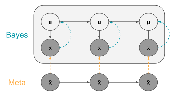 |
|---|
| Illustration of Bayesian learning via inference and meta learning via prediction. |
We will use the proof at the end of this paper. The idea is to show that the posterior predictive achieves higher likelihood than any other reference distribution \(r(x_{t+1}|x_{1:t})\):
or alternatively:
The proof proceeds as follow:
This proof seems kind of trivial in the sense that it mainly shows that the optimal predictor is the true model itself and it finds the best reference distribution in the forward KL sense. However, notice that I used the term “true model” rather loosely. In fact, what I meant was the true generative model \(P(x_{1:t+1}, \mu)\) which is not necessarily the same as the true posterior predictive \(P(x_{t+1}|x_{1:t})\), even though it is derived from the true generative model.
So one thing that would be useful to understand is whether there exists alternative predictive distributions that would yield the same predictions as the posterior predictive but are parameterized by different underlying generative models as the true generative model? In other words, whether the posterior predictive distribution is the unique solution to the problem and whether we can make the correct predictions for the wrong reason?
Can we make the correct predictions for the wrong reason?
Our goal is to find alternative generative models \(Q_{\theta}(\mu, x_{1:\infty})\) with parameters \(\theta\) who themselves are different from the true generative model but their posterior predictive distributions are equivalent to the ground truth generative model. Let us denote such a predictor parameterized by generative model as:
where \(b_{\theta}(\mu|x_{1:t})\) is the posterior distribution of the generative model \(Q_{\theta}(\mu, x_{1:\infty})\). The reason we still restrict ourselves to Bayesian reasoners (just with potentially wrong models) is that non-Bayesian reasoners can suffer from much more sub-optimality, which render them not worth considering in the context of making good predictions (see the Dutch book argument). However, the predictors do not have to be implemented as explicit Bayesian computation. For example, they can be implemented using amortized networks, such as recurrent neural networks (see this paper).
For this type of agent, it is helpful to think of its interaction (although no actions are involved) with the signal-generating environment as a Bayesian network where the ground truth \(\mu\) generates the observation \(x\) at every time step, and the agent’s belief \(b\) tracks the unknown \(\mu\) as each \(x\) is observed.
It is sufficient to analyze a single time slice of the Bayesian network, because if the predictive distribution based on the belief at any time step can be held fixed by varying the generative model parameters, then the solution is not unique. But it is worth noting that sometimes the condition required for such non-uniqueness may be increasingly strict when we increase the number of time steps, then the solution may ultimately be unique.
We will approach this analysis by computing the gradient of the predictor’s expected log likelihood with respect to the model parameters and check whether there could be more than set of one parameters for which the gradient is zero, which suggests non-uniqueness. Let’s denote the expected log likelihood for a single time slice as:
Recall that the gradient of log-sum-exp function is \(\nabla\log\sum_{x}\exp(f(x)) = \mathbb{E}_{\pi(x)}[\nabla f(x)]\), where \(\pi(x) \propto \exp(f(x))\), the log likelihood gradient is:
where \(\pi(\mu) \propto \exp(\log Q_{\theta}(x_{t+1}|\mu) + \log b_{\theta}(\mu|x_t)) = b_{\theta}(\mu|x_{t+1}, x_t)\) is the posterior under the parameterized generative model upon observing \(x_{t+1}\) and \(x_t\). We have also dropped the expectation over the observed data since it does not affect our analysis at this point.
We now apply a similar derivation to the second term in the gradient:
where \(\pi'(\mu) = b_{\theta}(\mu|x_t)\) for reasons similar to the previous step.
Plugging back to the previous equation, we have:
While the first line above is indeed very confusing, the second line has some interesting properties. The first term on the second line is the expected gradient of the log conditional likelihood of \(x_{t+1}\) under the current posterior. The second and third terms are the average log conditional likelihood of \(x_t\) and the average log prior weighted by the difference between the posterior beliefs at two adjacent steps. Let us make a reasonable assumption that the difference between beliefs at two adjacent steps becomes increasingly smaller for increasingly larger time steps, then, the log likelihood gradient reduces to the first term, which has to be equal to zero when the log likelihood is maximized.
Let us now make use of the ground truth generative distribution. We know that for each data sequence, the ground truth \(\mu\) is held fixed. Let us add a further assumption to the previous one that after observing enough samples, the belief distributions are not only similar across time steps, they are also highly concentrated in the sense that the model only has high belief on a single realization of \(\mu = \hat{\mu}\) (regardless of whether that is the correct one). Then, the first term in the gradient becomes approximately equal to \(\nabla\log Q_{\theta}(x_{t+1}|\hat{\mu})\) without the expectation. Then, we are essentially regressing \(x_{t+1}\) onto \(\hat{\mu}\) as if we have observed the ground truth (feels strangely like expectation-maximization right?). For sufficiently diverse context distribution, we will be able to perform this regression for every single realization of \(\mu\). As a result, \(Q_{\theta}(x_{t+1}|\mu)\) will approach the ground truth given enough data, up to a permutation of the semantics of \(\mu\).
This exercise shows not only that the optimal predictor for the current sequential prediction setting is the posterior predictive distribution of the ground truth generative model, but also that among all candidate predictors who are Bayesian reasoners with respect to some arbitrary generative models, only a single one corresponding to the ground truth generative model is optimal.
What if the context distribution is dynamically changing?
It is definitely satisfying to know that we can retrieve the ground truth generative model via meta learning when the context distribution is static. An intriguing question is whether this is still the case if the context distribution is allowed to change dynamically? This is a much more realistic setting. For example, the trend in the stock market over a period of time is usually not static.
Such a model can be written as:
where we have introduced a context transition distribution \(P(\mu_t|\mu_{t-1})\). This is in fact the classic hidden Markov model.
Let us consider a predictor which is parameterized by an arbitrary hidden Markov model. Its posterior predictive is:
Similar to the static case, we will analyze the gradient of its log likelihood for a single time slice:
where \(\pi(\mu_{t+1}) = b_{\theta}(\mu_{t+1}|x_{t+1}, x_t)\).
The second term above can be expanded as:
where \(m(\mu_t|\mu_{t+1}) \propto \exp(\log Q_{\theta}(\mu_{t+1}|\mu_t) + b_{\theta}(\mu_t|x_t)) = Q_{\theta}(\mu_t|\mu_{t+1}, x_t)\) is the inverse transition.
Expanding again the second term and using the results from the static case, we have:
where \(\pi(\mu_t') = b_{\theta}(\mu_t|x_t)\).
For the final term, we have:
where \(m(\mu_{t-1}|\mu_t) = Q_{\theta}(\mu_{t-1}|\mu_t)\).
Putting all together, the log likelihood gradient can be expressed as:
This result is similar to the static context case, where we have the expected conditional and transition likelihood and two additional terms quantifying the difference between the beliefs at two adjacent time steps. However, this time we cannot easily make the assumption that our belief will converge to a point given a large number of observations, because the context is always changing. In order to make the last two terms diminish and so that the solution is unique, we must require that either the context changes very slowly such that it is extremely unlikely that the belief changes substantially in a single step, or the context is easily recognizable, for example that context transition is deterministic and the conditional distributions are highly separated. The latter is the usual separability assumption in hidden Markov model identifiability. In practice, we may not need to require separability at all time steps but only at enough anchor points, since having easily recognizable context at all time steps seems to defeat the purpose of reasoning under uncertainty. Nevertheless, it seems useful to enforce some priors on the generative model parameters, for example for slowing changing context, to improve identifiability.
Identifiability in meta learning and Bayesian inference
While identifiability is a widely studied topic in Bayesian inference in the context of latent variable modeling, it has not gained as much attention in meta learning or even the more closely related Bayesian deep learning.
The Meta-learning of Sequential Strategies paper is perhaps one of the first to suggest the automatic emergence of Bayesian reasoning in meta learners. However, the authors did not make any strong arguments about the uniqueness of the solution. A subsequent paper empirically showed that hidden states of the meta learner’s recurrent network converge to the ground truth Bayesian sufficient statistics. Our excursion above suggests that this is indeed plausible.
Only until very recently have people started to be concerned about the identifiability of Bayesian deep learning methods, such as variational auto-encoders (VAE). For example, this paper suggests that VAEs are identifiable if the latent variables (i.e., our \(\mu\)) can be identified from data, and if this is not the case the model will suffer from posterior collapse, a well known issue in VAEs. The latent variable identifiability condition is precisely the separability assumption we mentioned previously. These issues have been known to exist in classic Bayesian models such as Gaussian mixture models and hidden Markov models.
Nevertheless, these questions are still worth studying because identifiability depends on the exact model and training setup. The question we raised about whether we can make the correct predictions with the wrong model is related to an old debate on discriminative training of generative models (or generative parameterization of discriminative models). Many models in this setting are not identifiable. But the meta learning setting seems to be identifiable thanks to the sequential nature of the task. This phenomenon is very interesting because many classical machine learners are not fans of discriminative training (see the same person on discriminative training). Some have even referred to neural networks trained based on pure predictive performance as “monference” for “model-inference pair”, or more to the point for “inference with no model”. But others have found exact one-to-one correspondence between RNN and HMM parameters. Overall, this might be more of a feature than a bug.
Before wrapping up, we should point out an important problem that has not been addressed: realizability, which will have immense implications for retrieving the underlying Bayesian networks in meta learners. So far we have assumed that the meta learner will actually learn to make optimal predictions, and if this is achieved, the underlying Bayesian network must be the unique true model. However, if the meta learner fails to achieve optimality, for example due to model capacity, data limitation, or optimization difficulty, then how do we understand the model being learned? In general, it is much more difficult to analyze suboptimal agents than optimal agents. As Leo Tolstoy says in Anna Karenina:
We will try to understand this in our subsequent excursions.