A Tutorial on Dual Reinforcement Learning - Mostly Intuitions

Most people think of reinforcement learning (RL) as online learning, trial-and-error learning, and sometimes minimizing reward prediction error. These views gave rise to and were also reinforced by the most popular algorithms, such as temporal-difference learning, policy gradient, etc. However, an alternative view of RL is data-driven optimization, where the RL process is one of the many possible means to the end goal of obtaining a near-optimal decision making policy in a dynamic environment that could only be (or sometimes better to) indirectly accessed via data samples (see Warren Powell’s book on this take).

Indeed, the most popular algorithm Q-learning represents the dynamic programming approach to optimization, which divides the sequential decision making problem into simpler subproblems, i.e., into non-sequential, 1-step optimization. While combining (neural network) function approximation and dynamic programming (a.k.a. DQN) has worked really well, it is also known to suffer from many issues and required specialized techniques to deal with. The issues are mostly due to finite sample size, distribution shift, and function approximator capacity which give rise to the common symptoms such as value over-estimation and the deadly triad.

Because of these issues with the approximate dynamic programming approach to RL, people have started exploring alternative approaches to optimizing policies. Dual RL is one such approach rooted in the linear programming formulation of sequential decision making problems. For every linear programming problem, there is a dual problem, which in some cases might be easier to solve than the original problem. Even if the dual problem is not immediately easier to solve, there might be additional tricks that can be applied.

The goal for this post is to rehearse some basic results on the state-of-the-art of dual RL from Nachum et al, 2020 and Sikchi et al, 2024 and demonstrate a toy example. At the end, we will see that the dual RL perspective applies convex duality to derive potentially better behaved Q-learning algorithms.

RL and linear programming

There are potentially many ways to formulate a sequential decision making problem in a Markov decision process (MDP; the main conceptual framework for RL) as a linear program (LP). The one which makes a clear connection with value-based dynamic programming is given by the following, along with its dual LP (see De Farias & Van Roy and this lecture):

$$ \begin{align} \text{Primal-V: } \max_{V} &\sum_{s}d_{0}(s)V(s) \\ \text{ s.t.} &V(s) \geq \max_{a \in \mathcal{A}}\left\{R(s, a) + \gamma\sum_{s'}P(s'|s, a)V(s')\right\}, \forall s \in \mathcal{S} \\ \text{Dual-V: } \max_{\rho \geq 0} &\sum_{s, a}\rho(s, a)R(s, a) \\ \text{ s.t.} &\sum_{a}\rho(s, a) = d_{0}(s) + \gamma\sum_{s', a'}P(s|s', a')\rho(s', a'), \forall s \in \mathcal{S} \\ \end{align} $$

where $d_{0}(s)$ is the initial state distribution, $R(s, a)$ the reward function, $P(s'|s, a)$ the transition dynamics, and $\gamma$ the discount factor.

It is clear that the constraint in Primal-V resembles the Bellman equation, and at optimality, we can interpret $V(s)$ as the optimal value function. In Dual-V, if we interpret $\rho(s, a)$ as the occupancy measure $\rho(s, a) = \mathbb{E}[\sum_{t=0}^{\infty}\gamma^{t}\Pr(s_{t}=s, a_{t}=a)]$, then the constraint can be read as the Bellman flow equation which says that the probability density or mass flowing into a state should equal that flowing out of a state.

Typically, the normalized or average occupancy measure $d(s, a) = (1 - \gamma)\rho(s, a)$ is considered in dual RL which simply divides both the objective and constraint by the effective planning horizon $\frac{1}{1 - \gamma}$. The objective is then interpreted as the average reward.

If we think of approximate dynamic programming as performing backward recursion (a.k.a. value iteration), then one of the reasons why it is not efficient is the curse of horizon (see this paper). To plan for a horizon of $H$, you will need to perform backward recursion $H$ times, usually for all states and actions. In this case, the dual view can be very appealing, because rather than performing a rigid number of iterations, we are searching in the space of occupancy measure which potentially has better structure to enable efficient search. The main question of course is how to solve it in a way that’s practical and admits sampling-based approaches to overcome the curse of dimensionality (due to large state and action space).

Why is it the dual?

For people who are not familiar with duality (like myself), it is not immediately clear what’s dualing. I will give a basic argument using the Lagrange multiplier, which we know is the primary approach to constrained optimization and the core component of Lagrangian duality. This will also clarify the meaning of different variables in the primal and dual problems.

For simplicity, we will consider a variation of the previous LP formulations:

$$ \begin{align} \text{Primal-Q: } \max_{\pi, Q} &\quad \sum_{s, a}d_{0}(s)\pi(a|s)Q(s, a) \\ \text{ s.t.} &\quad Q(s, a) \geq R(s, a) + \gamma\sum_{s', a'}P(s'|s, a)\pi(a'|s')Q(s', a'), \forall (s, a) \in \mathcal{S} \times \mathcal{A} \\ \text{Dual-Q: } \max_{\pi, \rho} &\quad \sum_{s, a}\rho(s, a)R(s, a) \\ \text{ s.t.} &\quad \rho(s, a) = d_{0}(s)\pi(a|s) + \gamma\sum_{s', a'}P(s|s', a')\rho(s', a')\pi(a|s), \forall (s, a) \in \mathcal{S} \times \mathcal{A} \\ \end{align} $$

where we remove the $\max$ in the constraint and introduce the policy $\pi(a|s)$. It is clear that $Q(s, a)$ resembles the state-action value function.

Here $\rho$ needs no nonnegativity constraint since we have $\vert\mathcal{S}\vert \times \vert\mathcal{A}\vert$ number of variables and the same number of constraints. As long as the MDP is well-behaved (i.e., matrix $I - \gamma P^{\pi}$ is invertible) then we have a unique solution for the system of equations. Since we know the unique solution is the occupancy measure, then $\rho$ must be equal to that and nonnegative.

To show how Dual-Q is related to Primal-Q, we write out the Lagrangian of Primal-Q where we introduce $\rho(s, a)$ as the Lagrange multiplier, one for each state-action pair:

$$ \begin{align} &L(\pi, Q, \rho) \\ &= \sum_{s, a}d_{0}(s)\pi(a|s)Q(s, a) \\ &\quad + \sum_{s, a}\rho(s, a)\underbrace{\left(R(s, a) + \gamma\sum_{s', a'}P(s'|s, a)\pi(a'|s')Q(s', a') - Q(s, a)\right)}_{\text{Primal-Q constraint}} \\ &= \sum_{s, a}\rho(s, a)R(s, a) \\ &\quad + \sum_{s, a}d_{0}(s)\pi(a|s)Q(s, a) + \sum_{s, a}\rho(s, a)\left(\gamma\sum_{s', a'}P(s'|s, a)\pi(a'|s')Q(s', a') - Q(s, a)\right) \\ &= \sum_{s, a}\rho(s, a)R(s, a) \\ &\quad + \sum_{s, a}Q(s, a)\underbrace{\left(d_{0}(s)\pi(a|s) + \gamma\sum_{s', a'}P(s|s', a')\rho(s', a')\pi(a|s) - \rho(s, a)\right)}_{\text{Dual-Q constraint}} \\ \end{align} $$

This shows that occupancy measure duals with value function: whereas occupancy measure serves as the dual variable in the primal problem, the value function serves as the dual variable in the dual problem.

Dual RL and control-as-inference

Reasoning about occupancy measure is such a fundamental twist on the RL problem (which usually reasons about value) that can be shown to be related to the control-as-inference framework (see Lazaro-Gredilla et al, 2024). This should not be too surprising after all, because control-as-inference reasons about the flipped question of what states and actions I should have experienced given I’m optimal.

To see the connection, recall that control-as-inference formulates RL as searching for a posterior distribution over trajectory $Q(\tau), \tau = (s_{0:T}, a_{0:T})$ which best explains the observation $\mathcal{O}_{0:T} = 1_{0:T}$ under the likelihood $P(\mathcal{O}_{t}=1|s_{t}, a_{t}) \propto \exp(\lambda R(s_{t}, a_{t}))$, where $\lambda \geq 0$ is a temperature parameter. The search objective can be written as the following variational lower bound:

$$ \begin{align} &\max_{Q \geq 0} \quad \mathbb{E}_{Q(\tau)}[\log P(\mathcal{O}_{0:T}|\tau)] - \mathbb{KL}[Q(\tau) || P(\tau|\pi)] \\ \propto &\max_{Q \geq 0} \quad \mathbb{E}_{Q(\tau)}[\sum_{t=0}^{T}R(s_{t}, a_{t})] - \frac{1}{\lambda}\mathbb{KL}[Q(\tau) || P(\tau|\pi)] \end{align} $$

where $P(\tau|\pi) = \prod_{t=0}^{T}P(s_{t}|s_{t-1}, a_{t-1})\pi(a_{t}|s_{t})$ is a prior over trajectories.

If we take $\lambda \rightarrow 0$, we can rewrite the above as the following constrained optimization problem:

$$ \max_{Q \geq 0} \quad \mathbb{E}_{Q(\tau)}[\sum_{t=0}^{T}R(s_{t}, a_{t})], \quad \text{s.t.} \quad \mathbb{KL}[Q(\tau) || P(\tau|\pi)] = 0 $$

Since the zero KL constraint only happens if $Q$ satisfy the marginal state-action probability, we can rewrite the above as:

$$ \begin{align} \max_{Q \geq 0} &\quad \mathbb{E}_{Q(\tau)}[\sum_{t=0}^{T}R(s_{t}, a_{t})] \\ \text{s.t.} &\quad \sum_{a_{t}}Q(s_{t}, a_{t}) = \sum_{s_{t-1}, a_{t-1}}P(s_{t}|s_{t-1}, a_{t-1})Q(s_{t-1}, a_{t-1}), \forall s_{t} \in \mathcal{S} \end{align} $$

It is clear that this is the finite horizon analog of the dual RL problem.

f-divergence and convex conjugate

The dual RL formulations introduced above aren’t actually easy to solve just yet. Indeed, the problems have a large (exponential) number of constraints and ensuring consistent Bellman flow is no easier (in my opinion harder) than ensuring consistent value functions. The main trick in SOTA dual RL relies on two theoretical tools called f-divergence and convex conjugate. However, typically no intuition is given when these tools are introduced in published papers. We will try to address this problem in this section.

f-divergence: f-divergence defines the statistical distance between two distributions $P$ and $Q$ using a convex function $f: \mathbb{R}_{+} \rightarrow \mathbb{R}$ as follow:

$$ \begin{align} D_{f}(P || Q) &= \mathbb{E}_{Q(z)}\left[f\left(\frac{P(z)}{Q(z)}\right)\right] \\ \end{align} $$

f-divergence generalizes a number of common divergences. For example, if we choose $f(x) = x\log x$, we get the reverse KL divergence:

$$ \begin{align} D_{f}(P || Q) &= \sum_{z}Q(z)\left(\frac{P(z)}{Q(z)}\log\frac{P(z)}{Q(z)}\right) \\ &= \sum_{z}P(z)\log\frac{P(z)}{Q(z)} \\ &= D_{KL}(P || Q) \end{align} $$

It is important to notice that $f$ is convex. This leads us to the next concept.

Convex conjugate: Let $f: \mathbb{R}_{+} \rightarrow \mathbb{R}$ be a convex function, its convex or Fenchel conjugate $f^{*}: \mathbb{R}_{+} \rightarrow \mathbb{R}$ is defined as:

$$ f^{*}(y) = \sup_{x \in \mathbb{R}_{+}}[x^{\intercal}y - f(x)] $$

This definition may seem very complex. One intuition is that for every given slope $y$ given as input, we will try to find a value $x$ such that the amount by which the linear function $y^{\intercal}x$ is greater than $f(x)$ is as large as possible (also see this tutorial by Mathieu Blondel). Since $f$ is convex, if the linear function intersects with $f$, this is the amount by which the linear function sits above the basin of $f$. If we move the linear function vertically to tangent $f$, then the difference become the intercept of the linear function on the vertical axis.

This intuition may not be that helpful just yet. So let’s consider KL divergence again where we define it as the function $f$:

$$ \begin{align} f(x) = D_{KL}(x || Q) = \mathbb{E}_{x(z)}[\log x(z) - \log Q(z)] \end{align} $$

To solve for its convex conjugate under the constraint that $x(z) = [x_{1}, ..., x_{|\mathcal{Z}|}]$ is a proper probability distribution with elements sum to 1, we take the derivative of the Lagrangian of the RHS and set to zero:

$$ \begin{align} \nabla_{x_{z}}L(x, \lambda) &= \nabla_{x_{z}}\left(x^{\intercal}y - \sum_{z}x_{z}(\log x_{z} - \log Q(z)) - \lambda (\sum_{z}x_{z} - 1)\right) \\ &= y - \log x_{z} + \log Q(z) - 1 - \lambda = 0\\ x_{z} &= \exp(y + \log Q(z) - \lambda - 1) \end{align} $$

Then to ensure $[x_{1}, ..., x_{|\mathcal{Z}|}]$ sums to 1, we have:

$$ \begin{align} \sum_{z}x_{z} &= \sum_{z}\exp(y(z) + \log Q(z) - \lambda - 1) \\ &= \frac{1}{\exp(\lambda)}\sum_{z}\exp(y(z) + \log Q(z) - 1) = 1 \\ \lambda &= \log\sum_{z}\exp(y(z) + \log Q(z) - 1) \\ &= \log\sum_{z}Q(z)\exp(y(z) - 1) \\ \end{align} $$

In other words, the Lagrange multiplier $\lambda$ becomes the log normalizer.

Plugging this solution into $f^{*}$, we have:

$$ \begin{align} f^{*}(y) &= y^{\intercal}\exp(y + \log Q - \lambda - 1) - \exp(y + \log Q - \lambda - 1)^{\intercal}(y + \cancel{\log Q} - \lambda - 1 - \cancel{\log Q}) \\ &= \exp(y + \log Q - \lambda - 1)^{\intercal}(\lambda + 1) \\ &= \sum_{z}\frac{\exp(y(z) + \log Q(z) - 1)}{\sum_{\tilde{z}}\exp(y(\tilde{z}) + \log Q(\tilde{z}) - 1)}(\lambda + 1) \\ &= \lambda + 1 \\ &= \log\sum_{z}\exp(y(z) + \log Q(z) - 1) + 1 \\ &= \log\sum_{z}\exp(y(z) + \log Q(z)) - \log e^{1} + 1 \\ &= \log\sum_{z}Q(z)\exp(y(z)) \end{align} $$

In other words, we have that the convex conjugate of the reverse KL divergence is the log-sum-exp function.

This is where the intuition comes in: if we let $y(z) = \log P(o|z)$ be the log likelihood of some observation $o$ given a latent state $z$, then we can interpret the log-sum-exp function as the log marginal likelihood of a simple latent variable model with prior $Q(z)$:

$$ \log\sum_{z}Q(z)\exp(y(z)) = \log\sum_{z}Q(z)P(o|z) = \log P(o) $$

We then see clearly what the convex conjugate is doing:

$$ \begin{align} \log P(o) &= \sup_{x}\sum_{z}x(z)\log P(o|z) - D_{KL}(x(z) || Q(z)) \\ &= \sup_{x}\mathbb{E}_{x(z)}[\log P(o|z)] - D_{KL}(x(z) || Q(z)) \end{align} $$

Now it all makes sense. In the case where $f$ is the reverse Kl divergence, the convex conjugate is the variational lower bound for any chosen log likelihood function. It does so by trying to find the best linear approximation to the conjugate under a concave penalty imposed by the negative of $f$.

In summary, for the family of f-divergence, convex conjugate can be seen as finding the variational representation of a marginalized score function for the chosen divergence measure.

RL under Lagrangian and Fenchel duality

The main trick to solving dual RL tractably, as proposed by Nachum et al, 2020 and Sikchi et al, 2024, is to use convex or Fenchel conjugate to convert the problem of satisfying an exponential number of constants into stochastic sampling, essentially by reversing the variational representation.

To do so, they propose a regularized formulation (from now on we use normalized occupancy measure $d(s, a) = (1 - \gamma)\rho(s, a)$):

$$ \begin{align} \text{Dual-Q: } \max_{\pi, d} &\quad \mathbb{E}_{d(s, a)}[R(s, a)] - \alpha D_{f}(d(s, a) || d^{O}(s, a)) \\ \text{s.t.} &\quad d(s, a) = (1 - \gamma)d_{0}(s)\pi(a|s) + \gamma\sum_{s', a'}P(s|s', a')d(s', a')\pi(a|s), \forall s \in \mathcal{S} \end{align} $$

where $d^{O}$ can be interpreted either as a distribution we want to regularized the solution against (e.g., an offline data distribution) or simply a data sampling distribution which we have access to. The parameter $\alpha$ controls the strength of the regularization and strictly generalizes the regular policy optimization problem which corresponds to $\alpha=0$.

We can write the Lagrangian dual of the inner problem as (i.e., policy evaluation, after scaling by $1/\alpha$):

$$ \begin{align} &\min_{Q}\max_{d} \quad \frac{1}{\alpha}\mathbb{E}_{d(s, a)}[R(s, a)] - D_{f}(d(s, a) || d^{O}(s, a)) \\ &\quad + \frac{1}{\alpha}\sum_{s, a}Q(s, a)\left\{(1 - \gamma)d_{0}(s)\pi(a|s) + \gamma\sum_{s', a'}P(s|s', a')d(s', a')\pi(a|s) - d(s, a)\right\} \\ &= \min_{Q}\max_{d} \quad \frac{(1 - \gamma)}{\alpha}\mathbb{E}_{d_{s}(s)\pi(a|s)}[Q(s, a)] - D_{f}(d(s, a) || d^{O}(s, a)) \\ &\quad + \mathbb{E}_{d(s, a)}\left[(R(s, a) + \gamma\sum_{s, a}P(s'|s, a)\pi(a'|s')Q(s', a') - Q(s, a))/\alpha\right] \end{align} $$

The last two terms highly resemble convex conjugate.

Let $y(s, a) = R(s, a) + \gamma\sum_{s, a}P(s'|s, a)\pi(a'|s')Q(s', a') - Q(s, a)$ (i.e., the Bellman error), we can write the last two terms above as:

$$ \begin{align} &\max_{d} \mathbb{E}_{d(s, a)}[y(s, a)/\alpha] - D_{f}(d(s, a) || d^{O}(s, a)) \\ &= \max_{d} \mathbb{E}_{d^{O}(s, a)}\left[\frac{d(s, a)}{d^{O}(s, a)} \frac{y(s, a)}{\alpha} - f\left(\frac{d(s, a)}{d^{O}(s, a)}\right)\right] \\ &= \mathbb{E}_{d^{O}(s, a)}\left[f^{*}(y(s, a)/\alpha)\right] \end{align} $$

The second line holds under what’s called the interchangeability principle, essentially due to the convexity of $f$.

We can then rewrite the dual problem as:

$$ \begin{align} \text{Dual-Q*: } &\max_{\pi}\min_{Q} \quad \frac{(1 - \gamma)}{\alpha}\mathbb{E}_{d_{0}(s)\pi(a|s)}[Q(s, a)] \\ &+ \mathbb{E}_{d^{O}(s, a)}\left[f^{*}\left(\frac{1}{\alpha}(R(s, a) + \gamma\sum_{s, a}P(s'|s, a)\pi(a'|s')Q(s', a') - Q(s, a))\right)\right] \end{align} $$

In other words, using convex conjugate we have replaced the inner problem of a min-max optimization with data sampling under a prior $d^{O}$ (though not quite the same as a prior). This also turns the problem into something similar to a regression problem with a special loss function. The loss function is in fact very interesting: it minimizes a convex function of the Bellman error while minimizing the Q function on the initial state distribution, effectively introduces a level of conservatism which we will see in the next section.

Maximum entropy RL Note that we can add an additional expected policy entropy term weighted by a temperature parameter $-\lambda \mathbb{E}_{P(s'\vert s, a)\pi(a' \vert s')}[\log\pi(a' \vert s')]$ to the objective function. Applying this to the Lagrangian dual, we get the soft-Bellman error instead of the Bellman error.

Telescoping initial state distribution The objective function can be a little problematic in that the first term is expected under the initial state distribution. If $d_{0}$ doesn’t have sufficient coverage of the state space, which is usually the case, it might reduce the learning signal for $Q$. Garg et al, 2021 presented a method for converting the expectation under $d_{0}$ into an expectation under an arbitrary distribution.

Specifically, let the arbitrary distribution be denoted as $\mu(s, a)$, we then have the following relationship:

$$ \begin{align} &\mathbb{E}_{\mu(s, a)}[V(s) - \gamma\mathbb{E}_{P(s'|s, a)}[V(s')]] \\ &= (1 - \gamma)\sum_{t=0}^{\infty}\gamma^{t}\mathbb{E}_{\mu_{t}(s, a)}[V(s) - \gamma\mathbb{E}_{P(s'|s, a)}[V(s')]] \\ &= (1 - \gamma)\sum_{t=0}^{\infty}\gamma^{t}\mathbb{E}_{\mu_{t}(s)}[V(s)] - (1 - \gamma)\sum_{t=0}^{\infty}\gamma^{t+1}\mathbb{E}_{\mu_{t+1}(s)}[V(s)] \\ &= (1 - \gamma)\mathbb{E}_{d_{0}(s)}[V(s)] \end{align} $$

In other words, it turns the initial state value into the difference between the value function at two adjacent time steps under an arbitrary distribution.

Set $V(s) = \mathbb{E}_{\pi(a|s)}[Q(s, a)]$, we can rewrite the first term in the Dual-Q problem as:

$$ (1 - \gamma)\mathbb{E}_{d_{0}(s)\pi(a|s)}[Q(s, a)] = \mathbb{E}_{\mu(s, a)}[\mathbb{E}_{\pi(a|s)}[Q(s, a)] - \gamma\mathbb{E}_{P(s'|s, a)\pi(a'|s')}[Q(s', a')]] $$

Connection with conservative Q-learning

An interesting property of this dual RL framework is that choosing difference f-divergence measures can recover different existing RL algorithms. Sikchi et al, 2024 listed several examples. One of them is CQL for offline RL.

Specifically, by choosing the $\chi^{2}$ divergence where $f(x) = (x - 1)^{2}$ and $f^{*}(y) = y^{2}/4 + y$, we can write the previous Dual-Q inner problem as:

$$ \begin{align} \min_{Q} \quad& \frac{(1 - \gamma)}{\alpha}\mathbb{E}_{d_{0}(s)\pi(a|s)}[Q(s, a)] + \frac{1}{\alpha}\mathbb{E}_{d^{O}(s, a)}[y(s, a)] + \frac{1}{4\alpha^{2}}\mathbb{E}_{d^{O}(s, a)}[y(s, a)^{2}] \end{align} $$

where the last term is just the expected squared Bellman error usually used in Q-learning.

Rearranging the first two terms (scaled by $\alpha$), we have:

$$ \begin{align} &(1 - \gamma)\mathbb{E}_{d_{0}(s)\pi(a|s)}[Q(s, a)] + \mathbb{E}_{d^{O}(s, a)}[R(s, a) + \gamma\sum_{s, a}P(s'|s, a)\pi(a'|s')Q(s', a') - Q(s, a)] \\ &= (1 - \gamma)\sum_{s, a}d_{0}(s)\pi(a|s)Q(s, a) + \sum_{s, a}\gamma d^{O}(s, a)\sum_{s', a'}P(s|s', a')\pi(a|s)Q(s, a) \\ &\quad - \mathbb{E}_{d^{O}(s, a)}[Q(s, a)] + \mathbb{E}_{d^{O}(s, a)}[R(s, a)] \\ &\propto \sum_{s, a}\left((1-\gamma)d_{0}(s)\pi(a|s) + \gamma d^{O}(s, a)\sum_{s', a'}P(s|s', a')\pi(a|s)\right)Q(s, a) - \mathbb{E}_{d^{O}(s, a)}[Q(s, a)] \\ &= \mathbb{E}_{d^{O}(s)\pi(a|s)}[Q(s, a)] - \mathbb{E}_{d^{O}(s, a)}[Q(s, a)] \\ \end{align} $$

where we have dropped the constant $\mathbb{E}_{d^{O}(s, a)}[R(s, a)]$.

Thus, the complete objective can be written as (scaled by $\alpha$):

$$ \max_{\pi}\min_{Q} \underbrace{\mathbb{E}_{d^{O}(s)\pi(a|s)}[Q(s, a)]}_{\text{min Q at OOD actions}} - \underbrace{\mathbb{E}_{d^{O}(s, a)}[Q(s, a)]}_{\text{max Q at in-dist actions}} - \underbrace{\frac{1}{4\alpha}\mathbb{E}_{d^{O}(s, a)}[y(s, a)^{2}]}_{\text{min Bellman error}} $$

which is exactly the CQL objective (Eq. 3).

An interesting property of this form of dual RL is that, despite similarity to standard actor-critic algorithms, the actor $\pi$ and critic $Q$ here optimize the same objective rather than two different objectives. In fact, as pointed out by Nachum et al, 2019, if $Q$ is optimized in the inner loop, the gradient of $\pi$ actually follows the on-policy gradient (under the f-divergence regularized Q function), effectively avoiding the deadly triad. It is thus interesting that the pessimism as captured by the first term might be an inherent property of aligned objectives in many contexts (see our paper on objective mismatch in RL).

Non-adversarial optimization in Dual-V form

A distinct advantage of dual RL is that the optimal occupancy measure can be obtained directly in the Dual-V from, without potentially unstable max-min optimization.

Recall the (regularized) Dual-V problem is:

$$ \begin{align} \text{Dual-V: } \max_{d \geq 0} &\quad \mathbb{E}_{d(s, a)}[R(s, a)] - \alpha D_{f}(d(s, a) || d^{O}(s, a)) \\ \text{s.t.} &\quad \sum_{a}d(s, a) = (1 - \gamma)d_{0}(s) + \gamma\sum_{s', a'}P(s|s', a')d(s', a'), \forall s \in \mathcal{S} \end{align} $$

Notice the policy $\pi$ is not present. Here we need the nonnegative constraint on $d$ because it cannot be uniquely determined by the Bellman flow constraints.

Similar to Dual-Q, we can write out its Lagrangian dual (scaled by $1/\alpha$):

$$ \begin{align} &\min_{V}\max_{d \geq 0} \quad \frac{1}{\alpha}\mathbb{E}_{d(s, a)}[R(s, a)] - D_{f}(d(s, a) || d^{O}(s, a)) \\ &\quad + \frac{1}{\alpha}\sum_{s}V(s)\left[(1 - \gamma)d_{0}(s) + \gamma\sum_{s', a'}P(s|s', a')d(s', a') - \sum_{a}d(s, a)\right] \\ &= \min_{V}\max_{d \geq 0} \quad \frac{(1 - \gamma)}{\alpha}\mathbb{E}_{d_{0}(s)}[V(s)] - D_{f}(d(s, a) || d^{O}(s, a)) \\ &\quad + \mathbb{E}_{d(s, a)}\left[(R(s, a) + \gamma\sum_{s'}P(s'|s, a)V(s') - V(s))/\alpha\right] \\ &= \min_{V}\max_{d \geq 0} \quad \frac{(1 - \gamma)}{\alpha}\mathbb{E}_{d_{0}(s)}[V(s)] \\ &\quad + \mathbb{E}_{d^{O}(s, a)}\left[\frac{d(s, a)}{d^{O}(s, a)}(R(s, a) + \gamma\sum_{s'}P(s'|s, a)V(s') - V(s))/\alpha\right] - \mathbb{E}_{d^{O}(s, a)}\left[f\left(\frac{d(s, a)}{d^{O}(s, a)}\right)\right] \\ &= \min_{V}\max_{w \geq 0} \quad \frac{(1 - \gamma)}{\alpha}\mathbb{E}_{d_{0}(s)}[V(s)] + \mathbb{E}_{d^{O}(s, a)}\left[w(s, a)y(s, a)/\alpha\right] - \mathbb{E}_{d^{O}(s, a)}[f(w(s, a))] \end{align} $$

where we have replaced $d$ with the importance ratio $w(s, a) = d(s, a)/d^{O}(s, a)$ which should also be constrained to be nonnegative and again $y(s, a)$ is the Bellman error. However, due to the nonnegative constraint, we can no longer apply convex conjugate directly.

To analyze the situation, let’s consider the Lagrangian dual of the inner problem:

$$ \min_{\lambda \geq 0}\max_{w \geq 0} \quad \mathbb{E}_{d^{O}(s, a)}\left[w(s, a)y(s, a)/\alpha\right] - \mathbb{E}_{d^{O}(s, a)}[f(w(s, a))] + \sum_{s, a}\lambda(s, a)w(s, a) $$

Basically, we want to solve this constrained problem in closed-form similar to what we did with reverse KL divergence, but for the general f-divergence family. The requirement of the solution being optimal (a.k.a. first-order condition) is that:

The gradient of the objective w.r.t. $w$ is zero,
$w(s, a) \geq 0, \lambda(s, a) \geq 0, \lambda(s, a)w(s, a) = 0, \forall (s, a) \in \mathcal{S} \times \mathcal{A}$.

The first bullet implies that:

$$ \begin{align} &d^{O}(s, a)^{\intercal}(y(s, a)/\alpha - f'(w(s, a)) + \lambda(s, a)) = 0 \\ &f'(w(s, a)) = y(s, a)/\alpha + \lambda(s, a) \end{align} $$

where $f'$ stands for the first derivative w.r.t. $f$’s argument.

The last requirement in the second bullet means that at optimality, the constraint should be inactive (a.k.a. complementary slackness) so that either $w(s, a) = 0$ or $\lambda(s, a) = 0$ (because this is the best choice for $\lambda$ if $w > 0$) or both. Thus the optimal $w$ is:

$$ w^{*}(s, a) = \max(0, f'^{-1}(y(s, a)/\alpha)) $$

where ${f'}^{-1}$ stands for the inverse of $f'$.

Plugging it back into the inner problem, we have:

$$ \begin{align} &\mathbb{E}_{d^{O}(s, a)}\left[w^{*}(s, a)y(s, a)/\alpha\right] - \mathbb{E}_{d^{O}(s, a)}[f(w^{*}(s, a))] \\ &= \mathbb{E}_{d^{O}(s, a)}\left[\max(0, f'^{-1}(y(s, a)/\alpha))y(s, a)/\alpha - f(\max(0, f'^{-1}(y(s, a)/\alpha)))\right] \\ &:= \mathbb{E}_{d^{O}(s, a)}[f^{*}_{p}(y(s, a)/\alpha)] \end{align} $$

Putting together, we have the Dual-V problem:

$$ \begin{align} \text{Dual-V*: } &\min_{V} \quad \frac{(1 - \gamma)}{\alpha}\mathbb{E}_{d_{0}(s)}[V(s)] \\ &+ \mathbb{E}_{d^{O}(s, a)}\left[f^{*}_{p}\left(\frac{1}{\alpha}(R(s, a) + \gamma\sum_{s'}P(s'|s, a)V(s') - V(s))\right)\right] \end{align} $$

which is a single regression-like problem. Some work also ignores the nonnegativity constraint, allowing us to directly use the convex conjugate.

Implicit maximization/policy improvement It is curious how, without any max or softmax operators, Dual-V* optimize the value function and thus the policy rather than just estimate the return or equivalently perform policy evaluation. The key is that it implicitly does so in the $f^{*}_{p}$ function. To see why, let’s write out $f^{*}_{p}$ in the piecewise format:

$$ \begin{align} f^{*}_{p}(y) = \left\{\begin{array}{ll} f'^{-1}(y)y - f(f'^{-1}(y)) = f^{*}(y) & \text{if } f'^{-1}(y) > 0\\ -f(0) & \text{otherwise } \end{array}\right. \end{align} $$

where $y$ is the Bellman error. Note that $f^{*}, f'^{-1}$ are strictly increasing functions (see visualizations here for example). Thus, the first line above roughly says that if the $f'^{-1}$ transformed Bellman error is positive, meaning the backed-up value function is higher than the predicted value function by some threshold, we will minimize the $f^{*}$ transformation of the error. If we use a semi-gradient update method, meaning stopping gradient on the backed-up value, then minimizing the second term corresponds to maximizing the predicted value until the threshold is met. For different chosen f-divergence, the threshold is different and some might be more amenable to optimization stability.

Recovering optimal policy While the Dual-V problem directly solves for the optimal value function, we need an additional step to retrieve the optimal policy. Luckily, we have the importance ratio under the optimal occupancy measure as an output:

$$ w^{*}(s, a) = \frac{d^{*}(s, a)}{d^{O}(s, a)} $$

We can then simply perform standard behavior cloning of the optimal actions by maximizing their log likelihood:

$$ \begin{align} \max_{\pi}\mathbb{E}_{d^{*}(s, a)}[\log \pi(a|s)] = \max_{\pi}\mathbb{E}_{d^{O}(s, a)}[w(s, a)\log \pi(a|s)] \end{align} $$

Alternatively, we can optimize the reverse KL which is slightly more involved. Check out Sikchi et al, 2024 if you are interested.

Imitation learning as regularized behavior cloning

An interesting byproduct of the f-divergence regularized formulation is that it puts RL and imitation learning (IL) on a spectrum where setting $\alpha \rightarrow \infty$ recovers IL via distribution matching. Adding a policy entropy regularization that is usually used in imitation learning, we can write the IL objective as follows:

$$ \begin{align} \text{IL-Q: } \max_{\pi, d} &\quad -D_{f}(d(s, a) || d^{E}(s, a)) + \mathbb{E}_{d(s, a, s')}[\lambda\mathbb{H}[\pi(a'|s')]] \\ \text{s.t.} &\quad d(s, a) = (1 - \gamma)d_{0}(s)\pi(a|s) + \gamma\sum_{s', a'}P(s|s', a')d(s', a')\pi(a|s), \forall s \in \mathcal{S} \end{align} $$

Applying the same steps as in Dual-Q but removing reward, we arrive at the following unconstrained IL problem:

$$ \begin{align} \text{IL-Q*: } &\max_{\pi}\min_{Q} \quad (1 - \gamma)\mathbb{E}_{d_{0}(s)\pi(a|s)}[Q(s, a)] \\ &+ \mathbb{E}_{d^{E}(s, a)}\left[f^{*}\left(\gamma\sum_{s, a}P(s'|s, a)V(s') - Q(s, a)\right)\right] \end{align} $$

where $V(s) = \mathbb{E}_{\pi(a|s)}[Q(s, a) - \log\pi(a|s)]$ is the soft value function. An important property of the optimal policy under entropy regularization is that its log likelihood can be written as $\log\pi(a|s) = \lambda(Q(s, a) - V(s))$.

Using $\chi^{2}$ divergence and the telescoping trick, we can expand the IL objective as:

$$ \begin{align} &\mathbb{E}_{d^{E}(s, a)}[V(s) - \gamma\mathbb{E}_{P(s'|s, a)}[V(s')]] + \mathbb{E}_{d^{E}(s, a)}\left[f^{*}\left(\gamma\mathbb{E}_{P(s'|s, a)}[V(s')] - Q(s, a)\right)\right] \\ &= \mathbb{E}_{d^{E}(s, a)}[V(s) - \cancel{\gamma\mathbb{E}_{P(s'|s, a)}[V(s')]}] + \mathbb{E}_{d^{E}(s, a)}\left[\cancel{\gamma\mathbb{E}_{P(s'|s, a)}[V(s')]} - Q(s, a)\right] \\ &\quad + \frac{1}{4}\mathbb{E}_{d^{E}(s, a)}[\left(\gamma\mathbb{E}_{P(s'|s, a)}[V(s')] - Q(s, a)\right)^{2}] \\ &= -\frac{1}{\lambda}\underbrace{\mathbb{E}_{d^{E}(s)}[\log \pi(a|s)]}_{\text{Behavior cloning}} + \frac{1}{4}\mathbb{E}_{d^{E}(s, a)}\underbrace{[\left(\gamma\mathbb{E}_{P(s'|s, a)}[V(s')] - Q(s, a)\right)^{2}]}_{\text{TD error}} \end{align} $$

The last line shows that imitation learning can be seen as TD-regularized behavior cloning. This method have recently been used by Wulfmeier et al, 2024 to perform language model supervised pre-training.

Toy example

We implement the above algorithms in the well-known mountain-car environment. A nice property about the mountain-car environment is that it’s dimensionality is low enough that the optimal policy after discretization can be computed in closed form as a comparison, but it is also complex enough that a random policy won’t do well. The code for the experiment can be found here.

One note about our implementation is that it is highly faithful to the derived objective function, where no coefficients are adapted ad hoc to accommodate the instability of neural nets (as done in Sikchi et al, 2024 ). This is not to say that our implementation is better, it’s more so that the environment is simple enough that no additional tricks are needed. The only other noteworthy thing is that we use semi-gradient updates in all places. This means that we stop the gradient on the target value (first two terms) in the Bellman residual as well as the second term in the telescoped initial value. Without semi-gradient updates, we were not able to achieve good results. If you look at the code here, the learning curves are actually quite unstable. This might be related to the conflicting gradient problem in the objectives, as highlighted by the recent ODICE paper.

On offline data distribution $d^{O}$, we use uniform sampling of the state-action space, although the distribution should in principle be generated from rollouts of data-collection policies. We tried data samples from higher entropy version of the optimal policy. However, that did not lead to value maps looking as pretty as the ones below. We believe this is most likely due to the reachability of the mountain-car environment.

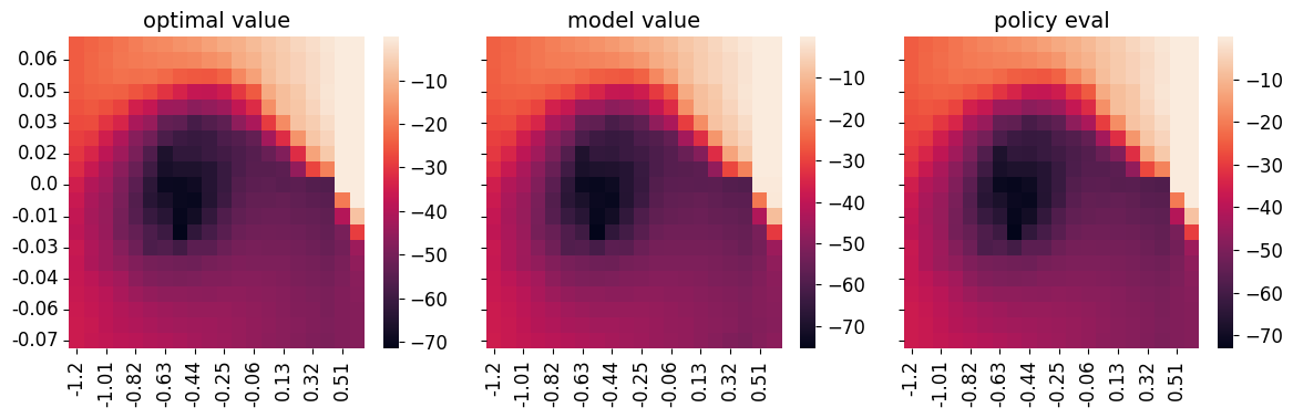
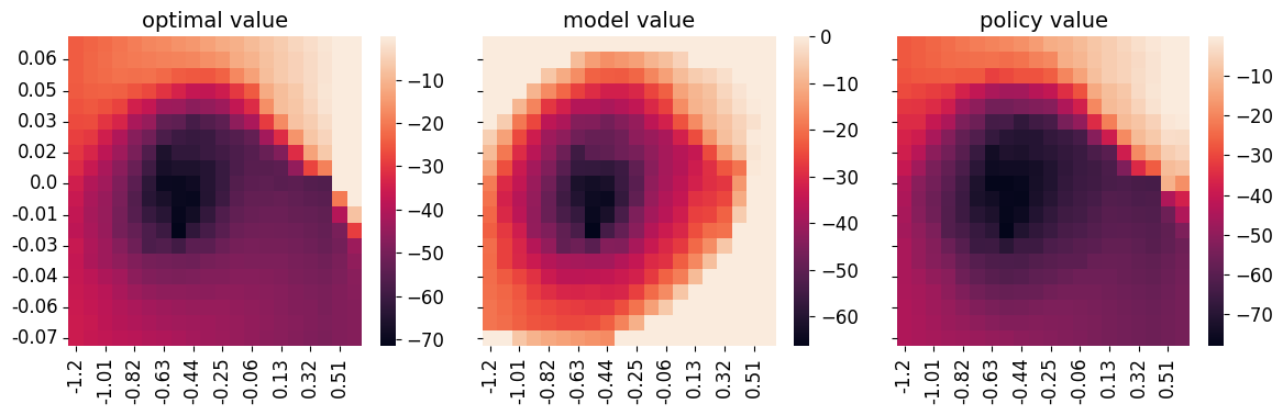
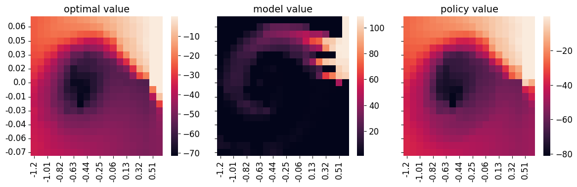
The results for Dual-Q, Dual-V and IL-Q* are shown below. The first column of all algorithms show the optimal value map as a comparison (x-axis is position and y-axis is velocity). The second column “model value” refers to the parameterized value function, which is a table in all cases. The last column “policy eval” is the expected value of the learned policy, a.k.a., policy evaluation which can be computed in closed form using the known transition matrix. All of the learned policies achieved near optimal performance when tested in the environment.

We see that Dual-Q* almost recover the ground truth optimal value map in both the learned value function and policy evaluation. For Dual-V, we see that the learned value has the correct pattern with low value in the middle, but it assigns high values to the border, somewhat incorrectly. This is likely related to the reachability of the mountain-car environment. Nevertheless, the policy evaluation map is pretty accurate. IL in this environment is pretty easy. Basically behavior cloning should be able to solve the task. We see that IL-Q has a pretty accurate policy evaluation map. The learned model value though is far from accurate compared to the ground truth. However, it does learn to assign high value to the goal state on the right, lower value in other states along the path, and lowest value to unreachable states. We can thus attribute the problem again to reachability and discretization and have some assurance that it won’t be the case without discretization or with smooth dynamics.


Dual-Q* values compared with optimal value.


Dual-V* values compared with optimal value.


IL-Q* values compared with optimal value.

Code availability Code to reproduce the experiments are available on Kaggle.

Acknowledgements The author would like to thank Harshit Sikchi for answering questions about dual RL.

References

- De Farias, D. P., & Van Roy, B. (2003). The linear programming approach to approximate dynamic programming. Operations research, 51(6), 850-865.
- Nachum, O., & Dai, B. (2020). Reinforcement learning via fenchel-rockafellar duality. arXiv preprint arXiv:2001.01866.
- Sikchi, H., Zheng, Q., Zhang, A., & Niekum, S. (2023). Dual rl: Unification and new methods for reinforcement and imitation learning. arXiv preprint arXiv:2302.08560.
- Garg, D., Chakraborty, S., Cundy, C., Song, J., & Ermon, S. (2021). Iq-learn: Inverse soft-q learning for imitation. Advances in Neural Information Processing Systems, 34, 4028-4039.
- Kumar, A., Zhou, A., Tucker, G., & Levine, S. (2020). Conservative q-learning for offline reinforcement learning. Advances in Neural Information Processing Systems, 33, 1179-1191.
- Wei, R., Lambert, N., McDonald, A., Garcia, A., & Calandra, R. (2023). A Unified View on Solving Objective Mismatch in Model-Based Reinforcement Learning. arXiv preprint arXiv:2310.06253.
- Wulfmeier, M., Bloesch, M., Vieillard, N., Ahuja, A., Bornschein, J., Huang, S., … & Riedmiller, M. (2024). Imitating Language via Scalable Inverse Reinforcement Learning. arXiv preprint arXiv:2409.01369.