Simple Alchemy for Meta Reinforcement Learning
This note aims to perform a detailed breakdown of the Alchemy environment developed by Deepmind in 2021 for meta reinforcement learning.
Short intro to meta RL The focus of meta RL, in contrast to regular RL, is fast adaptation to a distribution of tasks (think of different reward functions). This kind of adaptation is different from quickly learning a new policy from scratch. Instead, meta RL leverages the similarity between tasks in the distribution to extrapolate the agent’s existing expertise to new tasks, where existing expertise can be thought of as task-conditioned policies that have already been learned. In other words, the main job of the agent during adaptation is to infer the underlying task from new observations and reward signals (known as the task-inference approach to meta RL; see Luisa Zintgraf’s thesis).
The task-inference perspective highlights the fact that meta RL problems have a specific structure, which in fact can be subsumed under the broader framework of Bayesian RL and partially observable MDPs. Thus, to better understand the problem structures appearing in typical meta RL settings and benchmarks, I think it is a useful practice to write down the Bayesian networks of some of these problems.
Why Alchemy? I chose Alchemy because the problem structure appears to be sufficiently complex and yet its task distribution is discrete so that task inference can be performed in closed form. The problem is also structured in such a way that one could abstract away certain capabilities required to complete the task (e.g., object manipulation and local motion control) in order to focus on other strategic aspects (e.g., subgoal sequencing). For example, Alchemy offers two versions of the environment - an image-based environment and a symbolic environment - where in the latter image recognition and object manipulation capabilities are not needed. Lastly, the explanation in the original paper is a bit hard to understand, and the tutorial notebook in the repo is no longer maintained and has a version conflict in colab. Thankfully, there is another paper by Jiang et al, 2023 which has a much clearer description of a simplified symbolic Alchemy environment. So I hope this note can also contribute to making Alchemy more accessible.
My personal speculation is that Alchemy was a part of Deepmind’s effort to scale meta RL agents using large sequence models. After establishing the implicit Bayesian inference capability of meta RL agents in simple tasks such as multi-arm bandits , an environment was needed to test agent capabilities in much more complicated and realistic scenarios and validate more or less the same hypotheses. Alchemy was designed for this purpose as a diagnostic environment for meta RL agents, although it did not catch much attention after the publication. But the lessons learned ultimately led to the successful application of large transformer architecture to achieve human timescale adaptation in a much larger closed-source procedurally generated environment.
Breaking down Alchemy
At a high level, Alchemy is a set of object manipulation tasks where the agent needs to manipulate “stones” provided in the environment in order to complete certain requirements, and finally deposit the stones in a container called the caldron. The requirements are on the stone’s attributes, including size, color, and shape, which can be changed by dipping the stones in “potions”. The grasping, dipping, and depositing motions constitute local motion control.
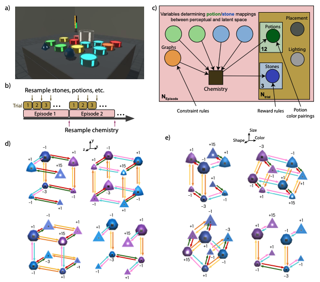
Panel a) in the figure below is a visualization of the environment. The gray triangle/pyramid on the left and gray ball near the middle of the image are the stones to be manipulated. The green, orange, yellow, and blue cylinders scattered around the table are the potions where the agent can dip the stones. The tall white cylinder in the center is the caldron which deposits the final stones.
 |
|---|
| Visualizations of the Alchemy environment, generative process, and causal graphs from the Alchemy paper. |
The goal of the agent is to transform the attributes of the stones by dipping them in the potions in order to manufacture stones with desired attributes, thus the name Alchemy. This requires “task-inference” because the effect of potions on the stones are governed by rules that are not directly revealed to the agent. However, once the agent has learned all the rules or the rules governing the creation of rules, it can dip the stones in some potions, as a form of experimentation, to figure out the underlying rule.
Specifically, the rules are represented as causal graphs (a.k.a. chemistry) shown in panel d) and e) of the figure above. We see that each node is a different combination of the stone attributes (\(size \in \{big, small\}\), \(color \in \{blue, purple\}\), \(shape \in \{round, triangle\}\)) and there are a total of 8 combinations. The arrows between the nodes represent the effects of the potions. There are a total of 3 pairs (or 6) potion colors, each pair has opposing/reversing effects. The fact that all arrows are on the outer edges of the cube means that each time a potion is applied, it can only change one attribute of the stones. In the figure, the brightness of the center of the stones represents their attractiveness or reward, which correspond to the annotated values -3, -1, +1 ,or +15. Also, notice that some shapes in the figure are neither round nor triangle, e.g., the blue stone with +1 reward in d) upper left. I’m not sure why that is the case exactly. It might be related to the section in the paper where they say even though each stone attribute has 2 potential values, their visual appearance may have one of the 3 predetermined values.
The episode structure is shown in panel b). Each episode consists of 10 trials with 20 steps each. Once a stone is deposited in the caldron, it counts towards the total reward at the end of the trial and cannot be retrieved. A random causal graph is sampled for each episode but fixed across all trials within the episode. In each new trial, the initial stone attributes and potion colors are randomly reset by the causal graph.
Causal graph generation
The causal graph generation process determines how many possible causal graphs, and thus tasks, the problem will have.
Given the above description, the causal graph generation process is pretty straightforward. In a similar spirit to Jiang et al, 2023, I will consider a simplified version of the symbolic environment, partly because I don’t know how the rewards are generated. For now I will just assume a certain attribute combination (e.g., big, blue, round) always has a reward of 1 while other attribute combinations have zero reward.
Given each stone always have 3 binary attributes, we can describe each attribute combination with a binary embedding of dimension 3: \(stone\_embedding \in \{0, 1\}^{3}\). Since each potion can only modify 1 attribute at a time, we can also describe it using an embedding of dimension 3 where the embedding values can take on \(\{-1, 0, 1\}\), however, only a single 1 or -1 can be present/activated at a time. The embeddings of each color pair have opposing activations. The effect of potion on stones can thus be described as addition of the two embeddings and clipping to range \([0, 1]\):
The variations in the causal graphs are introduced by random sampling of each potion pair’s effect on attributes and also whether the effects are applied on all edges. As shown in the figure above, each pair of potions can have effects on up to 4 edges. This is because for each target effect or target attribute, there are a maximum of 4 unique combinations of other attributes. The potion target attributes introduce 6 variations. The edge selections introduce 3375 variations (see code later). We thus have a total of 20250 causal graphs. This is an order of magnitude smaller than what’s calculated in the Alchemy paper, but sufficiently large for the simplified environment.
Task structure as Bayes net
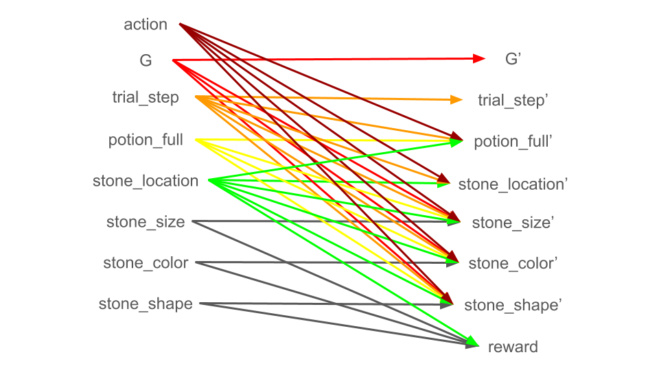
The main goal of the note is to write down the task structure or the task POMDP in the Bayesian network format. For simplicity, we consider 1 stone 6 unique potions as the setup in Jiang et al, 2023 rather than the 3 stones 12 potion setup in the original paper.
As a part of the background process, the episode and trial variables are time-based and do not depend on other variables. Assuming planning with infinite horizon and discounting, we will ignore trial numbers and focus on the time steps within each trial, which resets every 20 steps. We can write the transition of trial steps as follows:
The action space of this environment is discrete, which consists of do nothing, dip the stone in one of the potions, and deposit the stone in the caldron. Since the reward is only obtained if the stone is deposited in the caldron, we need to associate it with a location variable. At the beginning of each trial, the stone is initialized to be outside of the caldron. Once the stone is deposited in the caldron, it will remain there until the end of the trial. Thus, stone location depends on trial step and its current location. We can write this as:
The state of each potion can be described as either empty or full. The potions are reset as full at the beginning of each trial (or the last step of each previous trial), and once a potion is dipped while the stone is not in the caldron, it becomes empty. We can write this as:
The main logic of the game is that each dip in the potion changes the stone attributes, for which the rule is governed by the causal graph. However, the dipping action can only take effect if the chosen potion is not empty and the stone is not in the caldron. Furthermore, the attributes of the stone are randomly reset at the beginning of each trial. These conditions represent the dependencies of stone attributes which we group them into a variable \(x = [potion\_full^{1:6}, stone\_location, trial\_step]\) for notation clarity. Then we recognize that given these variables, the chosen action, and the causal graph \(G\), each stone attribute becomes conditionally independent:
Finally, the reward depends on the attributes of the stone and whether the stone is in the caldron:
We can visualize all these dependencies using the two time slice Bayesian network (2TBN) representation in the figure below.
 |
|---|
| Two time slice Bayesian network (2TBN) representation of the Alchemy environment. |
Solving Alchemy with MPC
The main goal of the exercise is to understand how well existing model predictive control (MPC) algorithms can solve the belief space planning problems required by meta RL tasks. Belief space planning is the optimal solution principle here because meta RL problems can be formulated as a special class of POMDPs for which there exists equivalent MDPs defined on the space of beliefs called belief MDPs (see my paper). The application of MPC which were developed for state space planning to this context is pretty straightforward as long as the belief MDP transition dynamics can be simulated. We use the cross entropy method (CEM) which is one of the most popular MPC algorithms in model-based RL.
Belief representation and updating
Given the discrete nature of the task distribution, we can perform belief updating in closed form using the Bayes rule:
Since size, color, shape and all variables in \(x\) from the last time step are already observed. We can directly index them in the likelihood distribution. In fact, we do not even need to explicitly parameterize other components of the Bayesian network other than just this distribution which contains the only variable \(G\) which needs to be inferred and memorized. For other distributions we only need to sample from them.
Belief space planning
For belief space planning, we need to be able to simulate the belief transition dynamics \(P(b'|b, a) = P(o'|b, a)\delta(b' - b'(o', a))\) for the CEM planner, where the second term denotes a delta distribution on a counterfactual Bayesian belief update given simulated future observation \(o'\).
Rewriting the posterior predictive as:
We can approximate this by drawing a single sample from the posterior predictive over state \(P(s'|b, a)\). Since the only latent state variable is the causal graph, this corresponds to drawing a random graph from the posterior and counterfactually updating the belief using the Bayes rule.
Results
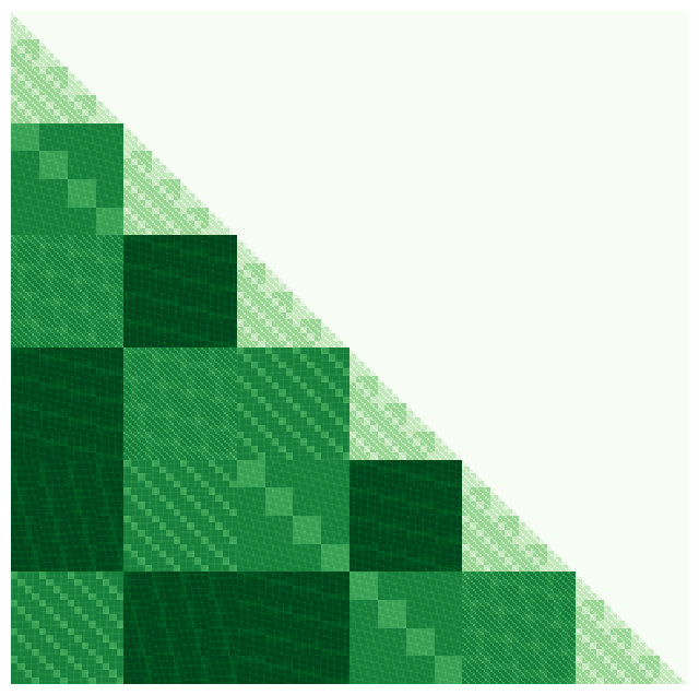
For simplicity, I only generated causal graphs with 3 edges for each stone attribute. This reduced the number of causal graphs from 20250 to 384. This makes planning much faster.
This figure below shows the similarity between every pair of causal graphs measured by the average KL divergence between their corresponding transition matrices. A nice sanity check is that it looks like there aren’t any pairs of causal graphs that have exactly the same transition matrices, i.e., zero KL divergence. However, the similarity matrix also shows that many causal graphs have the same dissimilarity. This means that there are many graphs which are slight permutations or modifications of one another, or alternatively, after observing the same sequence of stone attribute transitions, it may still be hard to narrow down the hypothesis to a single graph because of the invariance. This suggests that it might be much better to represent these hypotheses over graph structures in continuous latent embedding space as in Jiang et al, 2023 and other black-box sequence models rather than as distinct discrete objects as done here.
 |
|---|
| Causal graph similarity matrix measured by average KL divergence of each pair of causal graphs’ stone attribute transition matrices. |
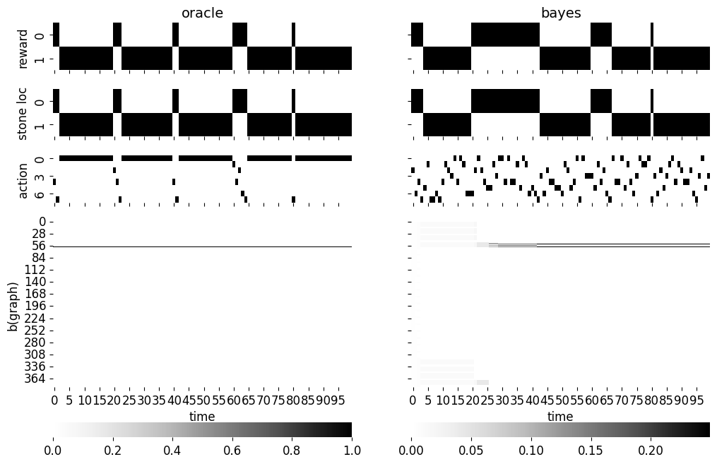
We compare the meta RL agent which performs explicit Bayesian inference (we thus call it the Bayes agent) over the latent graph structure with an oracle agent which has privileged access to the true graph structure. The oracle agent’s optimal policy can thus be computed in closed form using value iteration. For the Bayes agent, we can compute the posterior over graph structure in closed form but we perform belief space planning using CEM with a planning horizon of 20 steps, 500 particles, 100 elites, and 10 iterations. We run the simulation for a total of 4 trials or 100 steps.
We see that the Bayes agent eventually narrowed down the hypotheses to two main graph structures. However, even with such ambiguity and potential suboptimality from sample-based planning, it could still successfully complete most of the trials as shown by the reward pattern in the first row. The only trial it missed is the second trial. Although the experiment is far from conclusive, I think it gives some assurance on the potential of the MPC approach to meta RL.
 |
|---|
| Simulation of oracle agent with access to ground truth causal graph and Bayesian meta RL agent which performs inference over latent causal graph and policy search with CEM. |
Final thoughts
This is my initial exploration of a model-based approach to meta RL. There has been a large number of papers confirming the effectiveness of the model-free or black-box approach to meta RL where all one needs to do is to throw large enough sequence models to the problem (see this paper on RNN as strong baseline for meta RL and my previous post on the task identifiability of these black-box agents). But I think the model-based approach can still be very beneficial if you already have a model of the problem or environment, in which case there is no need to go through the slow RL process from scratch.
Perhaps one lesson from the experiment above is that model-based meta RL needs to get the task structure right so that limited memory capacity of the agent can be used effectively. This may also introduce an undesirable interaction with the MPC planner where the combinatorial explosion of the latent space might make the search process much more difficult for the planner. In this case, the search process may be modified to be better behaved with reward shaping such as using information-directed sampling (see my paper on this topic). However, in certain latent permutation invariant regimes as is the case in here, one needs to properly balance between information seeking vs tasking solving to prevent the agent from over-exploring useless information.
Code availability Code to reproduce the experiments are available on Kaggle.
References
- Wang, J. X., King, M., Porcel, N., Kurth-Nelson, Z., Zhu, T., Deck, C., … & Botvinick, M. (2021). Alchemy: A benchmark and analysis toolkit for meta-reinforcement learning agents. arXiv preprint arXiv:2102.02926.
- Jiang, C., Ke, N. R., & van Hasselt, H. (2023). Learning how to infer partial mdps for in-context adaptation and exploration. arXiv preprint arXiv:2302.04250.
- Team, A. A., Bauer, J., Baumli, K., Baveja, S., Behbahani, F., Bhoopchand, A., … & Zhang, L. (2023). Human-timescale adaptation in an open-ended task space. arXiv preprint arXiv:2301.07608.
- Ni, T., Eysenbach, B., & Salakhutdinov, R. (2021). Recurrent model-free rl can be a strong baseline for many pomdps. arXiv preprint arXiv:2110.05038.