RNNs are Switching State Space Models?
A recent paper introduced two new minimal variants of the classic recurrent neural network (RNN) architectures, GRU and LSTM. They show that these models offer a variety of benefits, including stable (no vanishing, exploding gradients) and fast (overfit faster than transformer) training and parallelizability using parallel scans.
An interesting observation is that, after removing concatenation and tanh activation, the new RNN cell update rules resemble message passing in switching dynamical systems, especially for minGRU. Let’s examine this a bit closer.
The classical GRU update rule is the following:
here \(\odot\) denotes element-wise multiplication. \(z\) and \(r\) represent a form of gating, preventing past information from being carried in the current hidden state. The gating decisions depend on both the previous hidden state and the current observation \(x_{t}\). Finally, the new (intermediate) hidden state \(\tilde{h}\) on the last line is a tanh-squashed linear transformation of the current observation and a gated previous hidden state.
Although the design choice of gating the previous hidden state based on the interaction between the hidden state and current observation via the concatenation is reasonable, not much can be said about this architecture from a (generative) modeling perspective, especially due to the tanh operator. Interestingly, these components are removed in the newly proposed minGRU update rules, which are written below:
We see that there is no more concatenation, and the new intermediate hidden state \(\tilde{h}\) only depends on the observation linearly.
It is now very tempting to interpret the update rules as a probabilistic generative model, because whenever we see weighted average using values between (0, 1) of the form in the first line, we think of expectation under Bernoulli random variables. Furthermore, the simple linear relationships make people think about log-linear models, which is the most common probabilistic model.
Log-linear models
To lay the groundwork, let’s first zoom in on the linear modules. The key idea here is that, assuming the outputs represent the logits of discrete categorical variables, linear operations can be read as either discriminative models as in logistic or softmax regression or generative models as the inversion or posterior of latent variable models:
Under the generative view, if \(x\) is a one-hot encoded categorical variable, then \(W\) and \(b\) can be interpreted as the likelihood and prior logits. If \(x\) is instead a continuous variables with Gaussian likelihood with different means \(\mu_{i}\) and shared variance \(\sigma\), in the simple case of \(y\) being a binary variable, the weights and bias can be interpreted as:
This is a well-known result on the equivalence between logistic regression and Gaussian naive Bayes classifiers (see this note).
Reverse engineering minGRU
Suppose we adopt the generative view, we can quickly obtain a tentative interpretation of minGRU:
where \(s\) denotes some supposed latent variables. Furthermore, since the RNN hidden states are set equal to the previous hidden states when \(z = 0\), we have \(\log P(s_{t}|x_{t}, z_{t}=0) = \log P(s_{t-1})\). In other words, \(z=0\) blocks off the propagation of information from \(x\) to \(s\). Since the weights and bias of \(linear(x)\) does not change over time, if there is a latent state transition distribution, then it should be of the form:
In other words, if \(z=0\), the latent state is a copy from a past state, otherwise, it is a new independent draw from a stationary distribution. We can then write a tentative version of the full generative model as:
This can be seen as a type of switching dynamical systems.
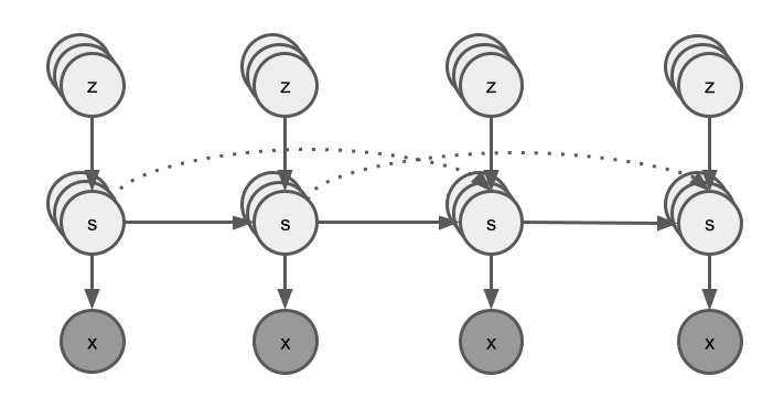 |
|---|
| Bayesian network of the switching dynamical systems interpretation of minGRU. Dashed lines represent copied-over latent variables when \(z=0\). |
If this is actually the generative model, then what should be the optimal posterior update rules in theory? Assuming we factorize the approximate posterior as \(Q(s, z|x) = Q(z|x)Q(s|x, z)\), the optimal update rules from variational message passing are the following:
So the choice of ignoring \(s\) in the updating of \(z\) in the minGRU interpretation can be understood as a generative model with very high mutual information between \(x\) and \(z\) such that observing \(x\) provides very precise information about \(z\) regardless of the values of \(s\).
Final thoughts
The analysis above only concerns a single layer RNN mapping from observations to latent states. If we stack multiple layers on top of each other, then the inferred latent states from the layer below become the observations from the layer above. Without applying a softmax operation between layer, the latent variable inference interpretation becomes a bit difficult in this setting.
Another observation is the assumption of independent draws at each step and carry over from earlier steps to later steps seems to make the network information too input driven and lacks inherent temporal dynamics. It is not clear whether this is problematic and in what setting.