Observations and Implementation Tricks for Imitation and Inverse Reinforcement Learning
While implementing the CleanIL repo, we found that certain algorithmic choices matter significantly for performance. By implementing a variety of algorithms, we also connected some conceptual dots and made some observations. In the spirit of The 37 Implementation Details of PPO, A Pragmatic Look at Deep Imitation Learning, and What Matters for Adversarial Imitation Learning?, we share these observations, tricks, and choices in this blog post. Unlike these larger scale prior works, we some of the observations maybe more anecdotal than systematic. Yet, we think it is worth being aware of them for practitioners.
Regularization of behavior cloning
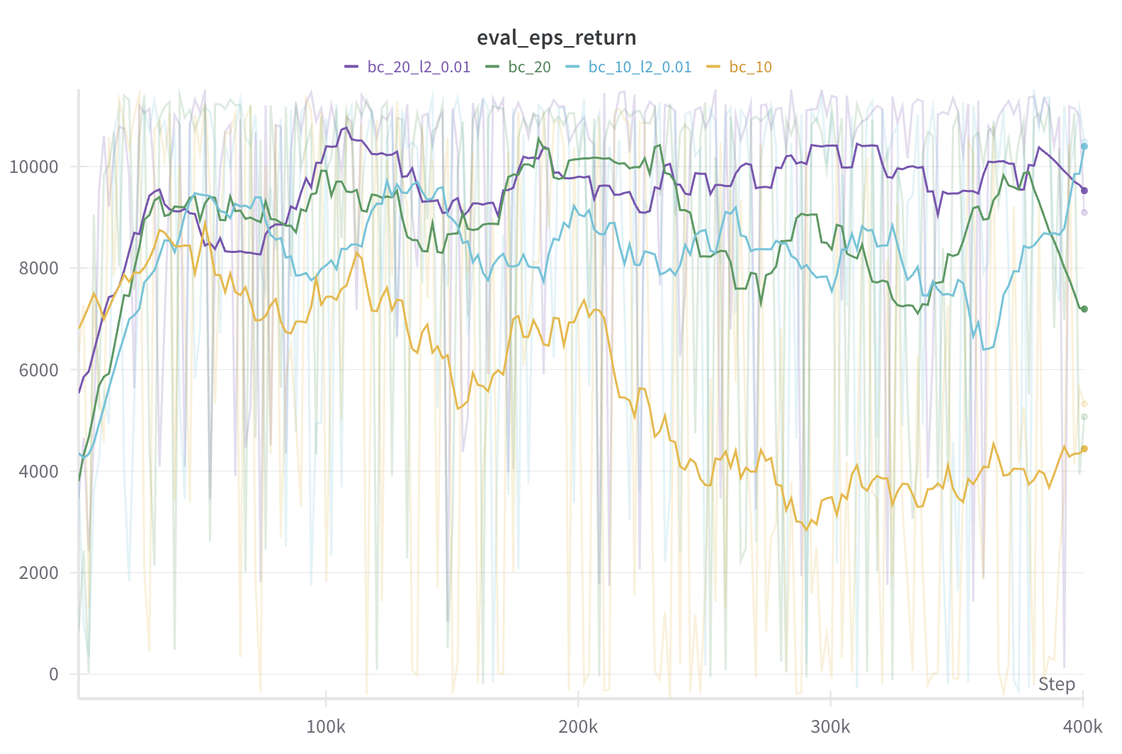
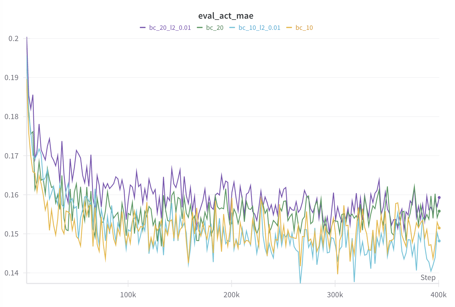
Empirically, many have observed that given enough data, behavior cloning achieves strong performance, often as strong as expert performance (see Fig. 1 in this paper for example.). Some even studied how specific data qualities, mostly related to data diversity and distribution coverage, contribute to BC performance. Besides data quality, Spencer et al, 2021 found that well optimized BC can achieve expert matching performance from just 25 expert trajectories in classic control and MuJoCo environments. Here, we show that l2 regularization on policy weights can substantially enhance performance with even 10 expert trajectories.
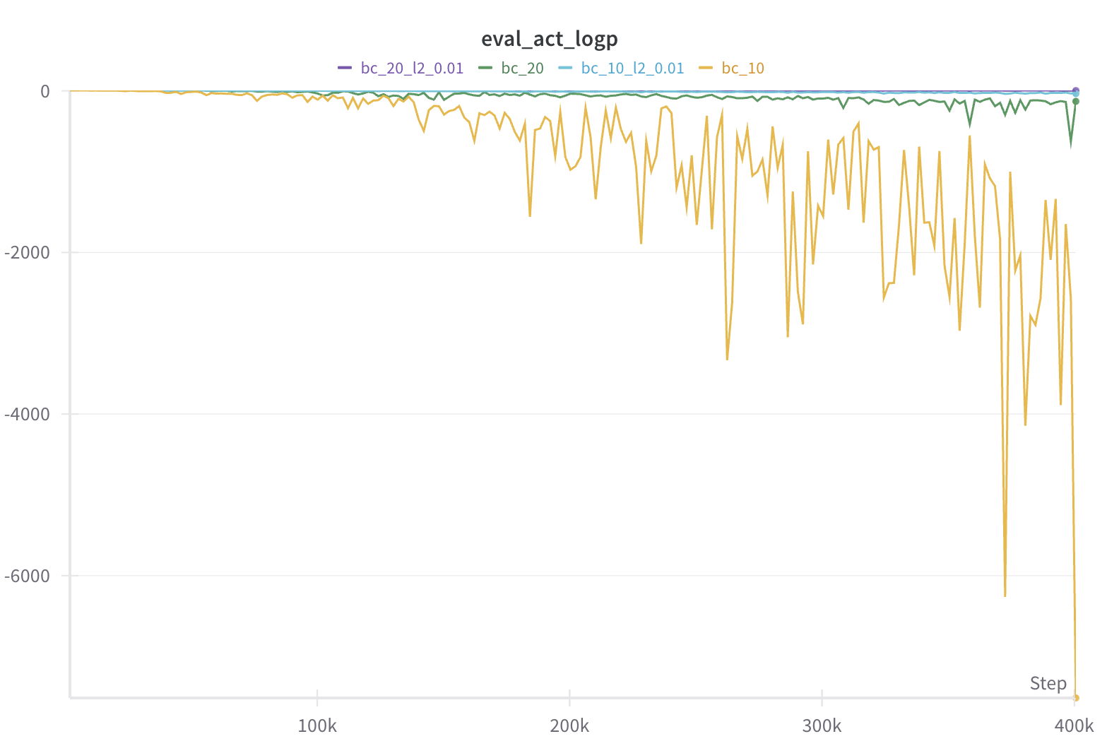
In the figures below, we plot the evaluation returns with moving average of 20 episodes in the first plot and mean average error (MAE) and log likelihood of evaluation set actions in second and third plots. We see that BC with 10 expert trajectories can reach 90% of expert performance quickly but soon deteriorates, which is mostly likely due to overfitting given extremely low log likelihood in the last plot. However, with l2 regularization with weight 0.01, we can more or less maintain the performance (see blue curve). l2 regularization also helps with slightly more data (20 expert trajectories; see purple curve), although the effect is less obvious.
 |
|---|
 |
 |
| Behavior cloning regularization comparision. |
A closer look at IQ-Learn and IBC
IQ-Learn and implicit behavior cloning (IBC) are two offline IL algorithms that learning a Q function or energy function from expert data instead of directly learning a policy. IBC was proposed to address complex action energy landscapes with discontinuities where commonly used parametric policies (e.g. Gaussian policies) may be misspecified and unable to fit these landscapes. IQ-Learn was proposed to bypass learning an intermediate reward function in regular adversarial IL which may be prone to instability. The realization here is that since the Q function is only trained on expert states in both algorithms, it would not know how to score actions on out-of-distribution states. Thus, they would suffer from the same issues as BC. This is supported by our evaluations where both IBC and IQ-Learn underperform BC.
This should be clear for IBC, given the negative samples drawn to optimize the info-NCE objective only randomized the actions but the states were still the same states in the dataset. However, this might be less obvious for IQ-Learn given its IRL root.
IQ-Learn proposes to replace the discriminator or reward function in adversarial IRL with an implicitly parameterized reward function using the the inverse Bellman operator:
This leads to the following IRL objective:
where \(f\) is a function related to the convex conjugate of f-divergences (see this tutorial on f-divergence and dual RL if interested).
To make this objective work with offline data, IQ-Learn leverages the property:
which replaces the potentially narrow initial state distribution \(d_{0}(s)\) with the stationary distribution \(\mu(s, a)\) of any policy.
Choosing \(\mu(s, a)\) to be the expert data distribution and the \(\chi^{2}\) divergence for \(f\), the resulting objective is a regularized version of IBC with a TD error penalty on the Q function:
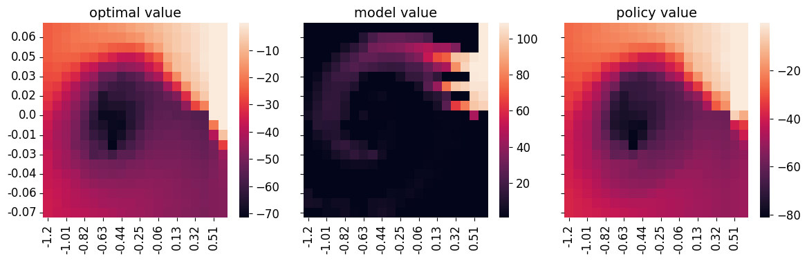
Issues with IQ-Learn: It is clear that the Q function is only trained on expert states and never on OOD states. So the critic does not know how to rank actions in OOD states. In the tabular setting, suppose we initialize the critic to be uniformly zero. Since the critic never receives any update on OOD states, the critic will remain uniformly zero in those states. This is in fact observed in our tabular experiment here (copied in figure below).
What IQ-learn will likely do? IQ-learn will likely learn to rank states along expert trajectories, where states at later time steps have higher value. This is because the TD objective \(Q(s, a) - \gamma\mathbb{E}_{P(s'\vert s, a)}[V(s')]\) forces \(Q(s, a)\) to be \(\gamma\) times the trailing state value. The ranking of states along expert trajectory is also observed in our tabular experiment. If the expert data actually has full coverage of the state-action space, then we can expect IQ-Learn to perform well and learn good Q functions. But this is rarely the case.
 |
|---|
| Tabular IQ-Learn on MountainCar results. |
Although the IQ-Learn objective generally makes sense if we look at IRL from a regularized BC perspective, how to regularize it and using what data does matters. One such objective with improved regularization is given by a recently proposed algorithm called RECOIL, which also learns a Q function using only offline data. Different from IQ-Learn, the RECOIL objective makes use of a suboptimal dataset \(d^{S}\) in the following objective function:
This objective makes much more sense because it uses an offline dataset which presumably has a larger coverage of the state-action space. Also, it uses the offline dataset in such a way that suboptimal state values are minimized while obeying TD regularization. This essentially creates a ranking over suboptimal states where states reachable from the expert states are assigned higher values so that when the agent stumbles upon these states, it knows to how to recover from them and return to expert states. Empirically, we see RECOIL achieving better performance compared to other BC based algorithms.
Actor critic vs AWR policy updates
Actor critic and advantage-weighted regression (AWR) are two ways to update the policy on off-policy and offline data. In AWR, we perform regression on potentially suboptimal actions in the offline data weighted by the estimated advantage. Actions with low advantage are correspondingly down weighted and not learned from. This makes policy optimization closer to supervised learning and intuitively we won’t do worse than the offline data. We found that BC based algorithms, such as IQ-Learn and RECOIL, significantly benefit from using AWR over soft actor critic (SAC).
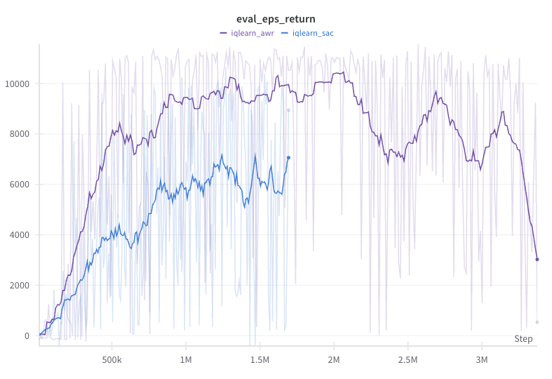
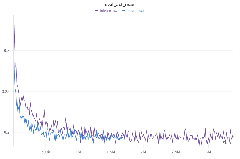
The figures below show that the SAC policy update method for IQ-Learn improves significantly slower than the AWR method and achieves lower performance asymptotically. This is despite the SAC method achieving lower MAE and higher log likelihood.
 |
|---|
 |
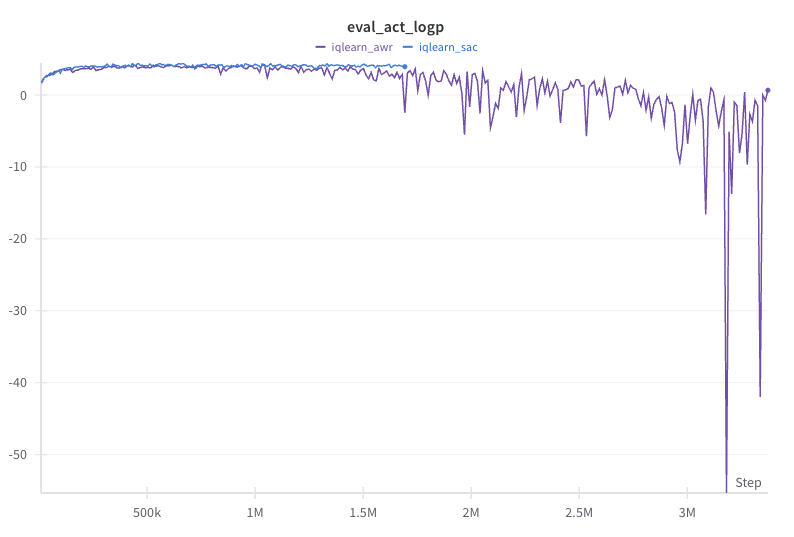 |
| IQ-Learn SAC vs AWR policy update comparison. |
Squared vs Huber TD loss
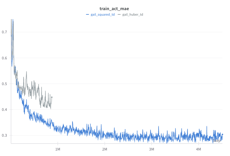
The squared TD error loss is the most common objective function for value learning in RL. However, for large TD errors, the squared loss can lead to very high loss values. For stability, some people have proposed to use the Huber loss, which transitions from squared loss to the l1 loss above some loss threshold. We found that for GAIL, the Huber loss does not work in the Hopper environment.
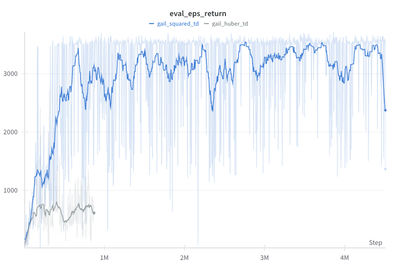
From the figures below, we see that despite some fast initial reduction in action MAE, the Huber loss version’s performance is stuck below 1000. One possible explanation is that the Huber loss does not penalize large TD errors as much as the squared loss. Yet, for the Hopper environment, getting the value of those states right is crucial to further learning. We did not experiment whether this could be mitigated by tuning the relative update ratio of value, policy, and reward.
 |
|---|
 |
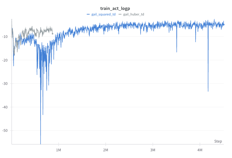 |
| GAIL squared vs Huber TD loss comparion in Hopper. |
For offline model-based algorithms such as OMLIRL and RMIRL, we decided to use Huber loss instead since initial error compounding in the learned dynamics rollout can lead to really high loss values and potentially hinder stability.
Different types of gradient penalties
Using gradient penalty (GP) on the discriminator or the reward function is the de facto method for improving training stability in adversarial IL and IRL, which is being used in almost all methods from GAIL to IBC. GP is widely studied in the related area of GAN, where different types of GP have been evaluated (for example see this paper). We list a few GP options used in the literature.
The original WGAN paper penalizes the deviation of the l2 norm of the discriminator from 1 on interpolated real and generated data:
This GP was adopted in for example F-IRL and RMIRL.
On the other hand, IBC uses a hinge loss so that the l\(\infty\) norm of the Q function is no higher than some threshold \(M\) on generated data:
We can understand these choices as the following:
- Squared loss vs hinge loss: whether we want the smoothness or Lipchitz constant of the reward function to be exactly 1 or less than or equal to some value.
- l2 vs l\(\infty\) norm: whether we want to force the smoothness property on the entire state-action space or alone each dimension.
- Interpolated vs non-interpolated data distribution: whether we want to force the smoothness property everywhere or only on expert or generated data distribution.
We think the hinge loss is less restrictive and applying it to interpolated data makes more sense. So this is the default option we have implemented.
Terminal state handling in offline model-based algorithms
The DAC paper pointed out that most IL and IRL algorithms do not properly handle terminal states and failing to do so can lead to a “survival bias” which may be undesirable in certain environments. This generally makes sense given that the terminal state should be modeled as a part of the state space. However, we found that including the terminal state may not be best for offline model-based algorithms.
The proposal in DAC is that we should add a binary terminal flag to the reward function. Given the expert data encounters fewer or no terminal states, while the initial learner data will encounter a lot more terminal states, the reward function will learn to assign low value to the terminal state and the policy will learn to avoid it. To allow the value function to properly learn on terminal states, they propose to add a self transition for every terminal state in the replay buffer. An alternative way to directly learn the correct terminal value as proposed by the LS-IQ paper is to compute it analytically using: \(\gamma/(1 - \gamma)R^{terminal}\).
For the two MuJoCo environments that have terminal states - Hopper and Walker2d - we found that it is sufficient to handle terminal state in the following way:
- Add binary terminal state flag to the reward function and mask out state-action input if the terminal flag is 1.
- Calculate the value function target in the regular way as:
reward + (1 - done) * gamma * v_next
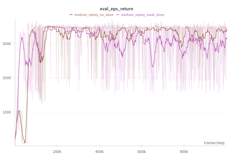
However, for the two offline model-based algorithms - OMLIRL which uses ensemble dynamics variance penalty and RMIRL which uses adversarial dynamics model fine-tuning - we found that although the terminal state flag has no effect on more expert trajectories or higher quality offline data (e.g. medium-expert), it can hinder performance when using fewer expert trajectories and lower quality offline data (e.g., medium-replay).
The figure below shows the evaluation performance of OMLIRL on the hopper-medium-replay-v2 dataset with 10 expert trajectories. We see that both versions with and without the done mask go through a stable stage at around 200k steps. However, the performance with the done mask starts to deteriorate after 400k steps, while the performance without the done mask remains stable.
One explanation is that the done mask makes the reward function too expressive. In the offline model-based setting, we set a state to the terminal state if the magnitude of the state features is above some threshold (this is to handle error compounding) and the value of some important state features falls out of the desired range (this is environment dependent; see implementation here). While in online IL, we can perfectly avoid terminal state at the end of training, this may not be possible in offline IL using learned approximate dynamics models. Thus, not using the done mask becomes a regularization technique to prevent the reward function from overfitting.
 |
|---|
| OMLIRL terminal state mask comparion on Hopper. |
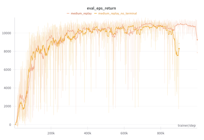
While the above is generally true, we found that both done mask and analytical terminal state value were needed for RMIRL in the HalfCheetah environment (see figure below). Specifically, without terminal state handling, RMIRL would improve and match expert performance for a while but then dramatically deteriorate at the end of training, by which point the value loss would blow up due to large magnitude of state features (feel free to check the benchmark wandb logs). We suspect this kind of behavior depends on how easily a learned dynamics model’s compounding error blows up. At which point we need to choose between the less poisonous of the two poisons of done mask vs complete crash.
 |
|---|
| RMIRL terminal state mask comparion on HalfCheetah. |
A few other implementation details for RMIRL:
- Adversarial model training: RMIRL uses RAMBO as the inner loop RL solver, both of which perform branched rollout from the offline dataset to reduce the expected value of sampled states with respect to the model parameters. However, in the original implementations, the branched rollouts ignore proper handling of terminal states. We found that this leads to the adversarial loss and thus subsequent value loss blowing up, mostly likely because the rollouts used for policy training always stop on terminal states so that the value function was never trained on states after terminal states and can be prone to over-extrapolation. We solve this by not stopping policy rollouts until the state magnitude is higher than some threshold and we use the same threshold in adversarial model training (see implementation here).
- Dynamics model training data: in the original paper of both RMIRL and OMLIRL, the authors trained the dynamics model on the offline dataset but excluded the expert trajectories. This was used to study the effect of distribution shift on offline model-based IRL where offline datasets with closer distribution coverage to the expert trajectories lead to higher performance. However, this was not ideal from a performance perspective given we have the expert trajectories at hand no matter how few. In our implementation, we add the 10 expert trajectories to the offline dataset for both dynamics model training and rollouts (we also experimented with upsampling the expert trajectories but it performed worse). It is clear that our performance on the medium-replay dataset substantially exceeds what’s reported in both papers.
To end the post, we hope these observations and implementation details are helpful for practitioners. Feel free to reach out if you have any questions!