Branching Reinforcement Learning
In this note, we explore an informal observation that the branching structure of data matters for policy or value learning in reinforcement learning, which is a more fine grained property than data distribution coverage used in most RL analyses.
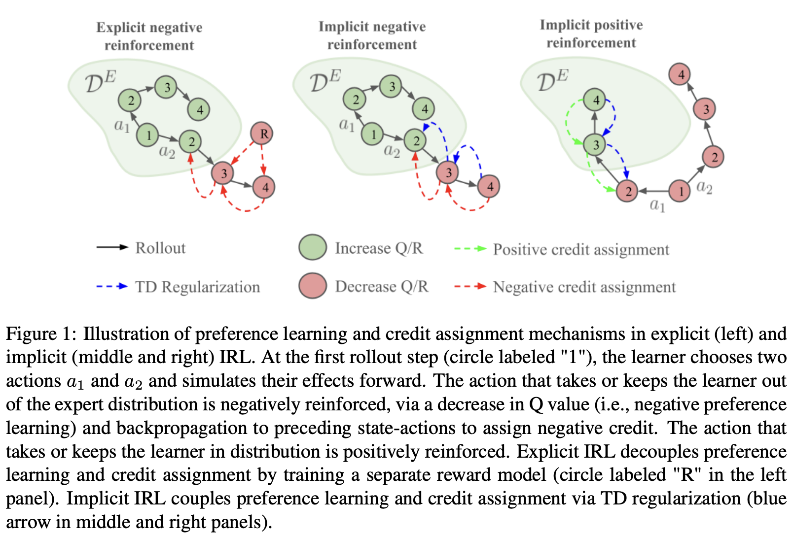
In 2025, I spent a good amount of time trying to understand the learning mechanisms underlying the so-called explicit and implicit inverse reinforcement learning (IRL) with the help of a few friends (see our paper here and a screenshot of the main takeaways below). I felt this understanding would be useful because implicit IRL is conceptually more scalable due to its structural similarity to behavior cloning; enhanced understanding would allow us to address its current shortcomings and make it more widely applicable. With some indirect experimental evidence, I found a few interesting properties of these IRL algorithms. First, in contrast to the idea that the more data the better, the learner policy gets the most signal from data branching away and towards the expert distribution to generate respectively negative and positive reinforcements, with negative reinforcement contributing more. Second, in implicit IRL algorithms that directly learn the Q function rather than the reward function, there is a mutual inhibition between preference learning and credit assignment, which makes the algorithm sensitive to hyperparameters.
 |
|---|
| Explicit vs implicit IRL learning dynamics from my paper. |
For the rest of 2025, I have been trying to prove these observations theoretically. Specifically, I have been looking for theoretical results that simultaneously address the optimality of implicit IRL (which can be compared to the optimality of explicit IRL in my previous paper), data branching properties, and preference learning-credit assignment inhibition. The task is a bit daunting, and, as of today, the overall progress has been slow.
Although nowhere near applicable to IRL, one subtask that I did make some progress on is data branching properties, which I believe is worth documenting. Given my previous proof for explicit IRL optimality is based on advantage function and density ratio correction, I continued along this direction. The key here is moving from marginal state-action density to state-action transition density. In this setting, the advantage function can be expanded in a temporal difference form, connecting the current state-action and the next state-action. This allows us to split the performance gap or regret of the learner policy into 4 partitions using the performance difference lemma; two of which arguably make the least contribution, and the remaining partitions correspond to the negative and positive reinforcement discussed above.
Bounding policy regret by data
Our goal here is to express the optimality of the learner policy \(\pi^{D}\) in terms of its training data \(D\). A typical approach is to compare the learner policy to a hypothetically optimal expert policy \(\pi^{*}\) and express its suboptimality by the performance gap from the expert. We denote the ratio between expert and data state-action density as \(w(s,a) = \frac{d^{\pi^{*}}(s, a)}{d^{D}(s, a)}\). It’s important to note here that just because the learner policy is trained on data \(D\) doesn’t mean it’s rollout density is or would be close to \(d^{D}\).
Using the well-known performance difference lemma, we can express the performance gap (a.k.a., regret) using the density ratio and the advantage function:
We can even bound the performance gap as:
with \(\Vert w(s, a)\Vert_{\infty} \leq C, \Vert A^{\pi^{D}}(s, a)\Vert_{\infty} \leq A_{max}\). Though this bound is not really that useful.
To introduce the idea of branching in the dataset, we define the following joint data distributions over a single step transition in addition to the previous marginal data distributions.
- Dataset joint: start in data occupancy, then branch following data policy
- Expert joint: start in expert occupancy, then branch following expert policy
- Mixed joint: start in expert occupancy, then branch following data policy
Let’s also define the one step on-policy temporal difference error:
Notice that the advantage function can be written in terms of this quantity experted under the dataset policy distribution:
The one step on-policy TD error represents branching in the following sense. If the learner policy takes an action \(a'\) that steers the agent to a worse state represented by low \(Q^{\pi^{D}}(s', a')\), then the TD error and advantage is negative. On the other hand, a positive TD error or advantage represents a positive branching, i.e., positive reinforcement or self-correction.
The joint density ratio between the mixed joint and the data joint can be defined as:
which turns out to be the same as the marginal density ratio.
We can use these quantities to express the performance gap using the performance difference lemma:
Naively, we can also bound the performance gap using these quantities:
which basically says regret is bounded by the expected TD error. Intuitively this makes sense, because zero TD error implies zero advantage.
Branching categories
The branching idea is that out of all partitions of the data, transitions from expert to suboptimal distribution or vise versa contributes the most to the learner policy performance. The other two data types, namely transitions within expert or suboptimal distributions matter less, especially the latter.
To explore this idea, we define the suboptimal marginal distribution \(d^{S}(s, a)\) and the suboptimal policy \(\pi^{S}(a|s)\), which we assume that generated the suboptimal parts of the dataset. Loosely, we say that these distributions have disjoint or very little overlapping support with the expert distributions. We then write the full data distributions as mixtures of expert and suboptimal distributions:
where \(\beta, \lambda\) are mixing weights. It is clear the joint transition data distribution is partitioned based on the initial state action distribution and the next action distribution. In practical settings, the dataset usually only contain a very small amount of expert data, so \(\beta\) and \(\lambda\) are generally very small.
A useful observation of the joint density ratio is the following:
If the expert and suboptimal distributions have nearly disjoint supports, then for \((s, a)\) in the expert support, \(w \approx 1/\beta\) which can be a large number, while for \((s, a)\) in the suboptimal support, \(w \approx 0\) because of zero density under expert distribution. This means that suboptimal start states and actions automatically have small contributions to performance.
We can now categorize all data into 4 partitions and analyze the importance weight and relative magnitude of the advantage in each partition of the data distribution:
Here, suboptimal start state contributions are automatically down weighted because of near zero importance weight, with suboptimal to suboptimal transition being the least useful. Transitions starting from expert states can be up-weighted by \(w \approx 1/\beta\). Because of the weighting, the first two data partitions have the largest contributions to policy performance.
The large negative advantage of the expert to suboptimal transitions are likely if the suboptimal policy points towards cliff states that cannot be recovered from. Similarly, suboptimal to expert transitions may generate large positive advantages if expert actions can undo cliff states.
A takeaway from this analysis is that it gives a more fine grained signal on data selection for RL than most existing analyses based on analyzing the marginal data distributions. Even though our importance weighting analysis shows that expert data still has the largest contribution to policy performance, which is consistent with existing analyses, it shows that how expert and suboptimal data are connected in terms of the MDP dynamics tree or reachability matters. Expert to suboptimal transitions are much more useful because of the large negative reinforcement they provide.
Simply concatenating expert and random data as done in many existing offline RL/IRL work is not ideal because it ignores how random data should be generated. What’s usually called medium-expert datasets empirically work much better likely because they better approximate the branching structure, assuming medium performance policy can reach some expert states but cannot do so consistently for the entire episode. The best way to generate branching data is to reset to states in the expert dataset and rollout from there, for which model-based approaches can be very handy.
Finally, we can obtain a simplified expression of the performance gap by keeping only high contribution terms:
Related work
The two main papers I have been referring to in this process are: When Should We Prefer Offline Reinforcement Learning Over Behavioral Cloning? Kumar et al, 2022 and A Dataset Perspective on Offline Reinforcement Learning, Schweighofer et al, 2021. The first paper derived several bounds for BC vs offline RL using a notion of critical state which is similar to my branching and cliff state idea. But I haven’t been able to adapt their technique to my setting. The second paper is more empirical but better captures my branching idea. They share a similar sentiment that combination of simple random data and expert data is not ideal for policy learning.